8. The Linear Regression Model
- 1 The Simple Linear Regression Model
- 2 The Multivariate Regression Model
- 3 Common Usage of the Multivariate Regression Model
- 4 Endogenous Regressors and Instrumental Variables
Most of the inferential statistics that we have dealt with so far treated statistical problems that arise when we observe a random sample of observations on a single random variable. In practice, most interesting questions deal with the effect that one (or more) variable(s) \(X\) has (or has not) on another variable \(Y\). The variable \(X\) is called a regressor and the variable \(Y\) is called the dependent variable. We will measure the effect of \(X\) on \(Y\) by the conditional mean function \(h(x)=E[Y|X=x]\). If \(X\) has no effect on \(Y\), this line would be horizontal.
To give a few examples, labour economists are interested in the effect that education has on wage and on the effect that class-size has on educational achievement. Macroeconomists are interested in the effect of investment and saving on the Gross Domestic Product of a country. Financial economists are interested in the effect of dividend payments on company valuations.
As most empirical work uses the linear regression model to answer these kind of questions, it is very important to get well-acquainted with it.
1 The Simple Linear Regression Model
As we consider two random variables \(X\) and \(Y\), the population distribution is now bivariate. As an example of a bivariate distribution, we consider a bivariate Normal distribution with means \(75\), variances \(100\) and covariance \(50\):
\[ \begin{bmatrix} X \\ Y \end{bmatrix} \sim N \left( \begin{bmatrix} \mu_y=75 \\ \mu_x=75 \end{bmatrix}, \begin{bmatrix} \sigma_{11}=100 & \sigma_{12}=50 \\ \sigma_{21}=50 & \sigma_{22}=100 \\ \end{bmatrix} \right) . \]
The bivariate density function and isoquants-graph are as follows:
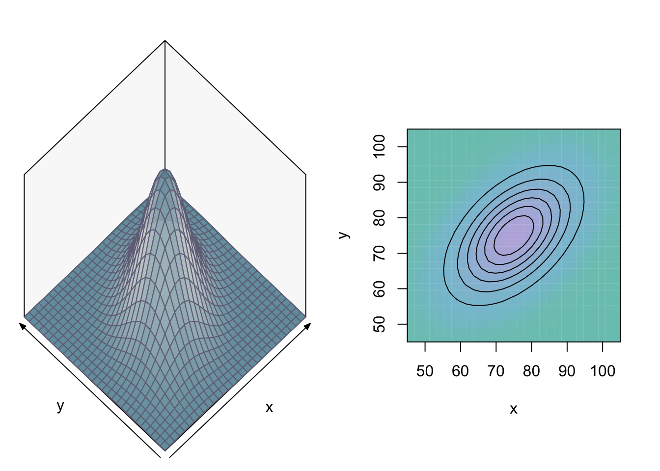
We will describe the effect of \(X\) on \(Y\) by the conditional mean function \(h(x)=E[Y|X=x]\), which returns the mean value of \(Y\) conditional on \(X=x\) (when we only consider the sub-population that has \(X=x\)). It can be shown that the conditional distributions from our bivariate Normal distribution have the following properties:
\[ \begin{align} Y | X=x &\sim N(E[Y|X=x], Var[Y|X=x]) \text{ (the conditional distributions are also Normal).}\\ E[Y|X=x] &= 37.5 + 0.5 x \text{ (the conditional mean function is linear).}\\ Var[Y|X=x] &= Var[\varepsilon|X=x]= \sigma^2_{\varepsilon} =75 \text{ (the conditional variance function is constant).} \end{align} \]
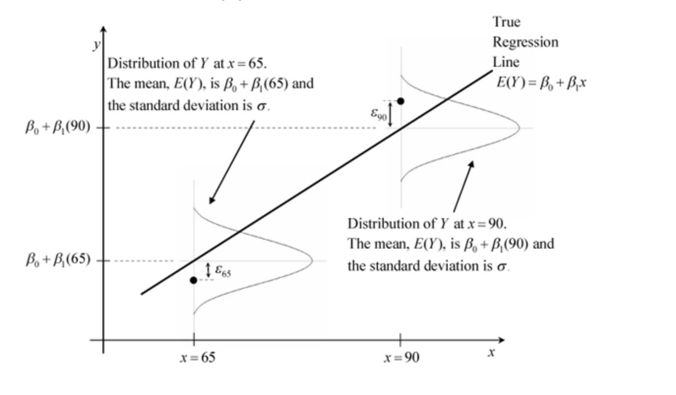
In the graph below, we focus on \(x=65\) (with \(E[Y|X=65]=70\)) and \(x=90\) (with \(E[Y|X=65]=82.5\)). Note that the line in the graph that connects the values of \(h(x)\) for all \(x\) is linear for this particular bivariate population distribution. Note also that the variance of the conditional distributions for this particular bivariate distribution is always \(\sigma^2_{\varepsilon}\), i.e. it is the same for all values of \(x\).
1.1 Linear Regression Model Assumptions
The assumptions of the linear regression model mimic the properties of the bivariate Normal distribution:
Assumption 1: Linear Conditional Mean Function
\[ E[Y|X=x]=\beta_0 + \beta_1 x \text{ for all values of }x. \]
This assumption is often stated in a different (but equivalent) way:
\[ y=\beta_0 + \beta_1 x + \varepsilon \text{ with } E[\varepsilon|X=x]=0, \]
where \(\varepsilon\) is the so-called disturbance or error. If a certain individual is the \(i^{th}\) observation in our dataset, its disturbance \(\varepsilon_i\) is equal to \(y_i - E[Y|X=x_i]\). A positive value of \(\varepsilon_i\) means that \(y_i\) is above average in the \(X=x_i\) sub-population. In the graph above, this occurs for the only individual for whom the values of \(x\) and \(y\) are plotted with \(x=90\). A negative value of \(\varepsilon_i\) means that \(y_i\) is below average in the \(X=x_i\) sub-population. In the graph above, this occurs for the only individual for whom the values of \(x\) and \(y\) are plotted with \(x=65\).
Assumption 2: Homoscedasticity
\[ Var[\varepsilon|X=x] = \sigma^2_{\varepsilon} \text{ (does not depend on }x). \]
As we cannot draw a linear line through a single point, we need variation in \(X\):
Assumption 3: No Multi-collinearity
\[ Var[X] \neq 0. \]
To obtain (exact) confidence intervals for \(\beta_1\) and to test hypotheses about \(\beta_1\) we need to assume more about the disturbance \(\varepsilon\):
Assumption 4: Disturbances are Normally Distributed
\[ \varepsilon | X=x \sim N(0, \sigma^2_{\varepsilon}), \]
or, equivalently, using the equation \(y=\beta_0 + \beta_1 x + \varepsilon\),
\[ Y | X=x \sim N(\beta_0 + \beta_1 x, \sigma^2_{\varepsilon}). \]
The graph above shows the conditional distributions of \(Y\) given \(x\) at \(x=65\) and \(x=90\). Note that assumption 4 includes the assumptions 1 and 2. Compared to assuming a bivariate Normal distribution, the only assumption that the linear regression model does not make is that \(X\) is Normally distributed. In the linear regression model, nothing is assumed about the distribution of \(X\) (apart from assumption 3). Its distribution can even be a discrete distribution.
Assumption 5: Our Sample is a Random Sample
This means that we take a random sample of people and we ask each person in the sample two questions. The answers of individual \(i\) are denoted by \((x_i,y_i)\). If the sample has size \(n\), we obtain a spreadsheet with two columns and \(n\) rows. The rows are \(n\) random draws from a bivariate population distribution. If we have time-series data, the random sample assumption is likely to be false: the time-series \(y=GDP\) and \(x=Inflation\) are both likely to be correlated over time.
1.2 The Ordinary Least Squares Estimator
The linear regression model assumes that the conditional mean function of the bivariate population distribution is linear. We do not observe the population distribution. All we observe is a random sample from the population distribution. This means that for \(n\) individuals (or firms/countries etc) we observe \((y_i, x_i)\), and that these pairs of observations are independent draws from the population distribution \(f_{Y,X}\).
We will estimate the constant and slope of the unknown conditional mean function by fitting a straight line that fits our sample-data best. Finding the best fitting line amounts to finding those values of \(\beta_0\) and \(\beta_1\) that minimise the sum of squared residuals function
\[ SSR(\beta_0,\beta_1)=\sum_{i=1}^n (y_i - (\beta_0 + \beta_1 x_i))^2. \]
The minimands are called the Ordinary Least Squares (OLS) estimators. As \(y_i\) and \(x_i\) are known values from our dataset, the sum of squared residuals function is is a function of two variables \(\beta_0\) and \(\beta_1\). The following animation illustrates the minimisation of SSR for the special case that \(\beta_0=0\), so only the slope needs to be estimated:
The sum of squared residuals function (\(SSR(\beta_1)\) in this case) is displayed on the right. It is evaluated in \(50\) different values of \(\beta_1\) and the sum of squared residuals function is minimal for the \(32^{th}\) value of \(\beta_1\): \(\beta_1=1.053\)
This trial-and-error approach can be replaced by calculus: the first derivatives are zero when evaluated in the arguments that minimise the function.
\[ \begin{align} &\frac{\delta SSR(\beta_0,\beta_1)}{\delta \beta_0} = 0 \Longleftrightarrow \\ & 2 \sum_{i=1}^n (y_i - \beta_0 -\beta_1 x_i) \times(-1) = 0 \Longleftrightarrow \\ & \sum_{i=1}^n y_i -n \beta_0 - \beta_1 \sum_{i=1}^n x_i = 0 \Longleftrightarrow \\ & \beta_0 = \bar{y} - \beta_1 \bar{x}. \end{align} \]
We will substitute this result into the first derivative of \(SSR(\beta_0,\beta_1)\) with respect to \(\beta_1\):
\[ \begin{align} &\frac{\delta SSR(\beta_0,\beta_1)}{\delta \beta_1} = 0 \Longleftrightarrow \\ & 2 \sum_{i=1}^n (y_i - \beta_0 -\beta_1 x_i) \times(-x_i) = 0 \Longleftrightarrow \\ & 2 \sum_{i=1}^n ( y_i - \bar{y} + \beta_1 \bar{x} - \beta_1x_i )(- x_i) = 0 \Longleftrightarrow \\ & 2 \sum_{i=1}^n ( \{y_i - \bar{y}\} + \beta_1 \{x_i - \bar{x}\})(- x_i) = 0 \Longleftrightarrow \\ & \sum_{i=1}^n ( y_i - \bar{y}\}x_i + \beta_1 \sum_{i=1}^n (x_i - \bar{x}) x_i = 0 \Longleftrightarrow \\ & \sum_{i=1}^n ( y_i - \bar{y})(x_i - \bar{x}) + \beta_1 \sum_{i=1}^n (x_i - \bar{x})^2 = 0 \Longleftrightarrow \\ & \beta_1 = \frac{\sum_{i=1}^n ( y_i - \bar{y})(x_i - \bar{x})}{\sum_{i=1}^n (x_i - \bar{x})^2}. \end{align} \]
The best fitting line through our data can therefore be found by calculating the OLS estimators for the constant and the slope:
\[ \begin{align} & \hat{\beta}_1^{ols} = \frac{\sum_{i=1}^n ( y_i - \bar{y})(x_i - \bar{x})}{\sum_{i=1}^n (x_i - \bar{x})^2}\\ & \hat{\beta}_0^{ols} = \bar{y} - \hat{\beta}_1^{ols} \bar{x} \end{align} \]
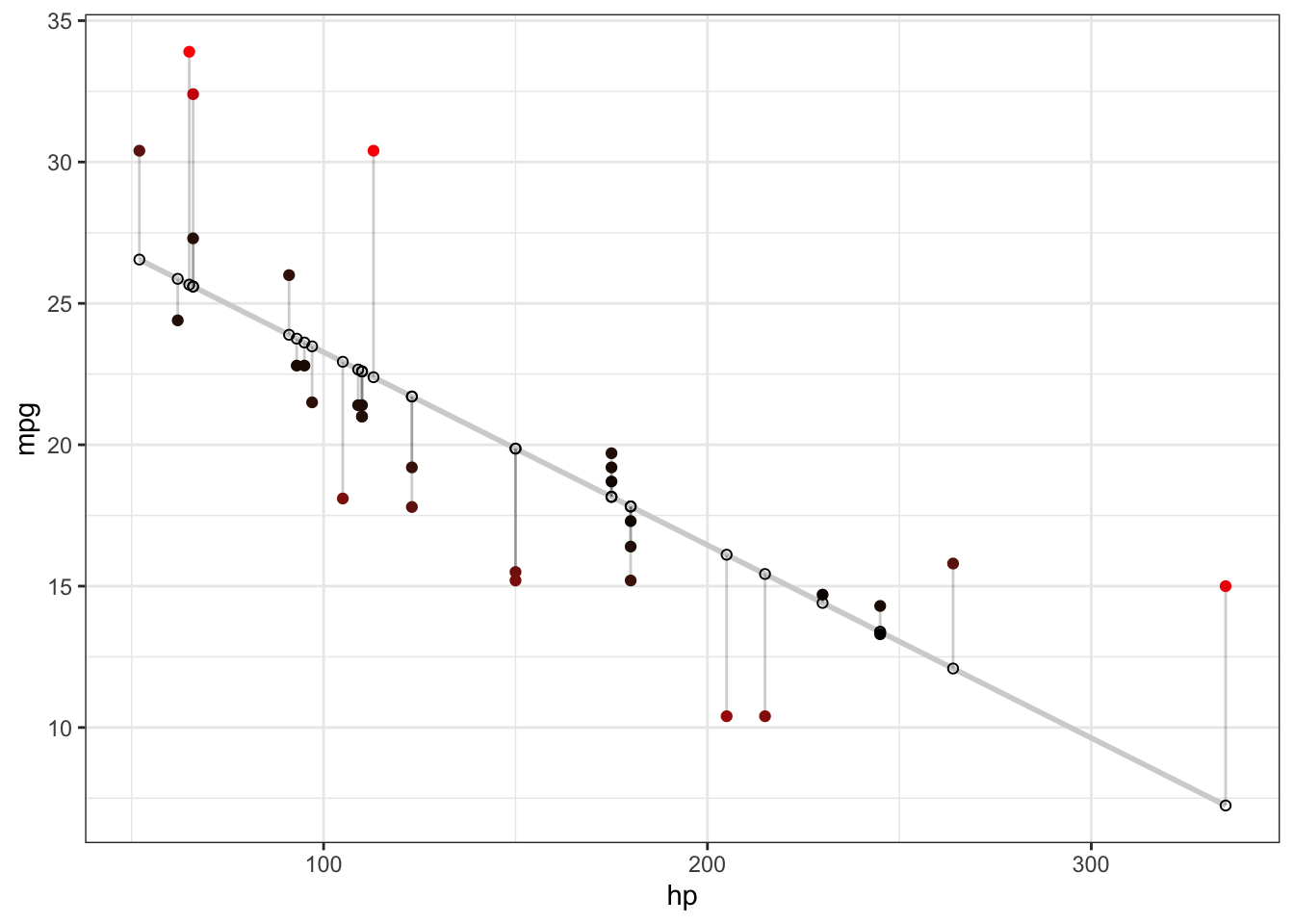
For any given dataset, we can have R calculate the OLS-estimators using the lm command. As an example, we estimate the effect of the horsepower of a car on its gasoline consumption (measured in miles per gallon of gasoline):
d <- mtcars
fit <- lm(mpg ~ hp, data = d)
summary(fit)
##
## Call:
## lm(formula = mpg ~ hp, data = d)
##
## Residuals:
## Min 1Q Median 3Q Max
## -5.7121 -2.1122 -0.8854 1.5819 8.2360
##
## Coefficients:
## Estimate Std. Error t value Pr(>|t|)
## (Intercept) 30.09886 1.63392 18.421 < 2e-16 ***
## hp -0.06823 0.01012 -6.742 1.79e-07 ***
## ---
## Signif. codes: 0 '***' 0.001 '**' 0.01 '*' 0.05 '.' 0.1 ' ' 1
##
## Residual standard error: 3.863 on 30 degrees of freedom
## Multiple R-squared: 0.6024, Adjusted R-squared: 0.5892
## F-statistic: 45.46 on 1 and 30 DF, p-value: 1.788e-07The residuals and predicted values can be calculated for each individual in the sample:
d$predicted <- predict(fit)   # Save the predicted values
d$residuals <- residuals(fit) # Save the residual values
## mpg hp predicted residuals
## Mazda RX4 21.0 110 22.59375 -1.5937500
## Mazda RX4 Wag 21.0 110 22.59375 -1.5937500
## Datsun 710 22.8 93 23.75363 -0.9536307
## Hornet 4 Drive 21.4 110 22.59375 -1.1937500
## Hornet Sportabout 18.7 175 18.15891 0.5410881
## Valiant 18.1 105 22.93489 -4.8348913We can now graph the data, the OLS-line containing the predicted values \(\hat{y}_i\), and the residuals \(\hat{\varepsilon}\):
1.3 The Coefficient of Determination \(R^2\)
We can assess the goodness of the fit by simply looking at the scatter plot that contains the estimated line. The closer the data are to the line, the better the fit. However, if we have 20 regressors, we will not be able to make a scatter plot of the data. It would be useful if we could construct a summary statistic that tells us how good the line (or plane) fits the data, and that can be calculated regardless of how many regressors we include in our regression model. The coefficient of determination \(R^2\) does exactly that. The coefficient of determination is defined as
\[ R^2 = \frac{ESS}{TSS} = 1 - \frac{RSS}{TSS}. \]
The terms \(TSS\), \(ESS\) and \(RSS\) are defined as follows: The total sum of squares \(TSS=\sum_{i=1}^n (y_i - \bar{y})^2\), and is hence a measure of the variability of the dependent variable \(y\). The explained sum of squares equals \(ESS = \sum_{i=1}^n (\hat{y}_i - \bar{y})^2\). The residual sum of squares \(RSS=\sum_{i=1}^n (y_i - \hat{y}_i)^2\) is the quantity that OLS minimises. The second equality follows because, as we will show later, \(TSS = ESS + RSS\). This equality also implies that \(ESS \leq TSS\) because \(TSS \geq 0\) as it is a sum of squares. Therefore, \[0 \leq R^2 \leq 1.\] If \(R^2\) is close to one, the regression models fits the data very well. If \(R^2\) is close to zero, the regression model does not fit the data at all very well.
The equality \(TSS = ESS + RSS\) can be derived as follows:
\[ \begin{align} TSS &= \sum_{i=1}^n (y_i - \bar{y})^2 \\ &= \sum_{i=1}^n \left\{ (y_i - \hat{y}_i) + (\hat{y}_i - \bar{y}) \right\}^2 \\ &= \sum_{i=1}^n (y_i - \hat{y}_i)^2 + 2 \sum_{i=1}^n (y_i - \hat{y}_i)(\hat{y}_i - \bar{y}) + \sum_{i=1}^n (\hat{y}_i - \bar{y})^2 \\ &= RSS + 0 + ESS \\ &= ESS + RSS. \end{align} \]
The fact that the cross-product equals zero is not shown and is also not obvious. It can be shown using two properties of the OLS residuals: \(\sum_{i=1}^n \hat{\varepsilon}_i = 0\) and \(\sum_{i=1}^n x_i \hat{\varepsilon}_i = 0\).
The explained sum of squares ESS deserves some further explanation: The simplest possible regression model that you can choose is the model \(y_i = \beta_0 + \varepsilon_i\), a model without any regressors except the constant. The sum of squared residuals for this model equals
\[SSR(\beta_0) = \sum_{i=1}^n (y_i - \beta_0)^2.\] The value of \(\beta_0\) that minimises this function is \(\hat{\beta}_0^{ols}=\bar{y}\). This simple model therefore has predictions \(y_i = \bar{y}\) for all individuals \(i = 1,2, \ldots,n\). The model estimates the unknown conditional mean function of the population distribution by a horizontal line through the data (with value \(\bar{y}\)).
A model with \(x\) added as a regressor may well give rise to better predictions \(\hat{y}_i = \hat{\beta}_0^{ols} + \hat{\beta}_1^{ols} x_i\). As \(ESS = \sum_{i=1}^n (\hat{y}_i - \bar{y})^2\), the value of ESS becomes larger if the predictions from our regression model \(\hat{y}_i\) are very different from the predictions of the simplest possible model that has predictions \(\bar{y}\). The more the additional regressor \(x\) explains, the higher the value of ESS and (because TSS is always the same) the lower the value of RSS. It is for this reason that \(R^2\) is defined as \(\frac{ESS}{TSS}\): it is the fraction of TSS that can be attributed to ESS, the explanatory power of the regressor \(x\).
1.4 Interpretation of the Estimation Results
We use the hprice1 dataset from the wooldridge package as an example.
1.4.1 Models in Levels
Consider the following estimated linear regression model:
\[ \hat{y}_i = \hat{\beta}_0^{ols} + \hat{\beta}_1^{ols}x_i. \]
The interpretation of \(\hat{\beta}_0^{ols}\) is as follows:
It is estimated that, for units with \(x=0\), \(E[Y|X=0]=\hat{\beta}_0^{ols}\).The interpretation of \(\hat{\beta}_1^{ols}\) is as follows:
It is estimated that if I increase \(x\) with \(1\) unit, \(y\) increases (on average) with \(\hat{\beta}_1^{ols}\).
The reason why the slope \(\beta_1\) has this interpretation is as follows: as \(E[Y|X=x]=\beta_0 + \beta_1 x\), we have that
\[ \beta_1 = \frac{d E[Y|X=x]}{dx}. \]
What a unit is depends on how the variables in the dataset are measured: if \(x=income\) is measured in Euros, then a unit is one Euro. If it is measured in thousands of Euros, one unit is 1000 Euros.
1.4.2 Models with Logarithms
You will often find regression results where either the dependent variable and/or one or more regressors are in logarithms instead of levels. Although we can interpret our parameter estimates in the normal way, it is more convenient to use a slightly different way of interpreting the parameters in this case. For example, we could interpret our estimate of \(\beta_{1}\) in the model \[\begin{equation} y=\beta_{0}+\beta_{1}\ln x+\epsilon\label{eq:semilog} \end{equation}\]
as the (average) change in \(y\) given a one unit change in \(\ln x\). This interpretation is problematic because it is not obvious what the change in \(x\) needs to be in order to change \(\ln x\) with one unit. The necessary change actually depends of on the value that \(x\) (and hence \(\ln(x)\)) has before increasing \(\ln(x)\) with one unit. It is more convenient in this case to interpret the estimation results using percentage-changes. The percentage-change interpretations are given in the Table below. These interpretations can be understood by first noting the following facts:
If \(x\) changes from \(100\) to \(120\), the change in \(x\), denoted by \(dx\), is \(20\). In that case, \(x\) has increased by \(20\%\). The percentage change in \(x\) is therefore \(20\). Any percentage change can likewise be calculated as \(100\left(\frac{dx}{x}\right)\).
A function \(f(x)\) can be linearly approximated around a given expansion point \(x_{0}\) by \(f(x)\approx f(x_{0})+f^{\prime}(x_{0})\left(x-x_{0}\right)=L_{x_{0}}(x)\). The linear approximation function \(L_{x_{0}}(x)\) is usually expressed in the form \(df_{x_{0}}(x)=\left.f^{\prime}(x)\right|_{x=x_{0}}dx\), where \(df_{x_0}(x)\) denotes \(L(x)-L(x_{0})\) and \(dx\) denotes \(\left(x-x_{0}\right)\). The references to the expansion point \(x_{0}\) are usually omitted. Applying this to the function \(\ln(x)\), we obtain \(d\ln(x)=\frac{1}{x}dx\). This means that if \(x\) changes with \(dx\), the linear approximation of \(\ln(x)\) (denoted by \(d\ln(x)\)) changes with \(\frac{1}{x}dx\).
Now, consider the regression model \(y=\beta_{0} + \beta_{1}\ln(x) + \epsilon\). Together with \(E\left[\epsilon|\ln(x)\right]=0\), this regression models states that \(E\left[y|\ln(x)\right]=\beta_{0}+\beta_{1}\ln(x)\). The parameter \(\beta_{1}\) can hence be interpreted as \(\beta_{1}=\frac{dE\left[y|\ln(x)\right]}{d\ln(x)}\). This corresponds to the normal interpretation: if \(d\ln(x)=1\), the average change in \(y\) is \(\beta_{1}\). We can rewrite this statement (using fact number \(2\) above) as \(\beta_{1}=\frac{dE\left[y|\ln(x)\right]}{\frac{1}{x}dx}\), which can itself be rewritten in terms of \(100\left(\frac{dx}{x}\right)\), the percentage-change in \(x\): \[\begin{alignat*}{1} \frac{\beta_{1}}{100}= & \frac{dE\left[y|\ln(x)\right]}{100\left(\frac{1}{x}dx\right)}. \end{alignat*}\]
This means that if \(x\) changes with \(1\%\) (i.e. if \(100\left(\frac{1}{x}dx\right)=1\)), \(y\) changes (on average) with \(\frac{\beta_{1}}{100}\) units. The other results in the Table can be obtained by using the same logic, except for case 3b which will be discussed in the section “Models with Dummy Variables” below.
The 5 different interpretations of \(\beta_{1}\) in regression models with or without logarithms are:
| Number | Name | Model | Interpretation of \(\beta_{1}\) |
|---|---|---|---|
| 1 | level-level | \(y=\beta_{0}+\beta_{1}x+\epsilon\) | If I increase \(x\) with \(1\) unit, \(y\) increases (on average) with \(\beta_{1}\). |
| 2 | level-log | \(y=\beta_{0}+\beta_{1}\ln(x)+\epsilon\) | If I increase \(x\) with \(1\%\), \(y\) increases (on average) with \(\frac{\beta_{1}}{100}\). |
| 3a | log-level | \(\ln(y)=\beta_{0}+\beta_{1}x+\epsilon\) | If I increase \(x\) with 1 unit, \(y\) increases (on average) with \(100\beta_{1}\%\). |
| 3b | log-dummy | \(\ln(y)=\beta_{0}+\beta_{1}D+\epsilon\) | If I increase \(D\) with \(1\) unit, \(y\) increases (on average) with \(100\left(e^{\beta_{1}}-1\right)\%\). |
| 4 | log-log | \(\ln(y)=\beta_{0}+\beta_{1}\ln(x)+\epsilon\) | If I increase \(x\) with \(1\%\), \(y\) increases (on average) with \(\beta_{1}\%\). |
In case 3b, the regressor is not a continuous but a discrete (dummy) variable, so \(\beta_{1}\) cannot be interpreted as a derivative. Instead, we need to use the ``discrete derivative’’ (difference), in that \[\begin{eqnarray} \beta_{1} & = & \underbrace{E\left[\ln(y)|D=1\right]}_{\beta_{0}+\beta_{1}}-\underbrace{E\left[\ln(y)|D=0\right]}_{\beta_{0}}\equiv y_{1}-y_{0}=\ln(\tilde{y}_{1})-\ln(\tilde{y}_{0}),\label{eq:beta1-in-case-3b} \end{eqnarray}\]
for some (unique) values \(\tilde{y}_{1}\) and \(\tilde{y}_{0}\) that satisfy \(y_{1}=\ln(\tilde{y}_{1})\) and \(y_{0}=\ln(\tilde{y}_{0})\).
If \(y\) denotes wage and D is a female-dummy, the normal way of interpreting \(\beta_{1}\) would read: the logarithm of wage is (on average) \(\beta_{1}\) higher for females compared to males. It would be easier to interpret the estimation results in terms of the level of wages (\(\tilde{y}\)), as opposed to the logarithm of wages (\(y\)). A change in average \(\ln(wage)\) from \(y_{0}\) to \(y_{1}\) corresponds to a change in wage from \(\tilde{y}_{0}\) to \(\tilde{y}_{1}\). We can now rephrase the interpretation of \(\beta_{1}\) into a statement that uses the percentage change in wage that occurs when we move from \(\tilde{y}_{0}\) to \(\tilde{y}_{1}\). Equation implies that \[\begin{align} \beta_{1} & =\ln\left(\frac{\tilde{y}_{1}}{\tilde{y}_{0}}\right)=\ln\left(\frac{\tilde{y}_{1}-\tilde{y}_{0}}{\tilde{y}_{0}}+1\right)\Longleftrightarrow\\ e^{\beta_{1}} & =\frac{\tilde{y}_{1}-\tilde{y}_{0}}{\tilde{y}_{0}}+1\Longleftrightarrow\\ e^{\beta_{1}}-1 & =\frac{\tilde{y}_{1}-\tilde{y}_{0}}{\tilde{y}_{0}}\Longleftrightarrow\\ 100\left(e^{\beta_{1}}-1\right) & =100\left(\frac{\tilde{y}_{1}-\tilde{y}_{0}}{\tilde{y}_{0}}\right)=100\left(\frac{d\tilde{y}}{\tilde{y}}\right). \end{align}\]
Therefore, a difference in average \(\ln(wage)\) of \(\beta_{1}\) corresponds to the female wage being \(100\left(e^{\beta_{1}}-1\right)\%\) higher than the male wage.
3a is a first-order (linear) Taylor approximation of 3b
A differentiable function \(f(x)\) can be linearly approximated in the neighbourhood of (the expansion point) \(x_{0}\) by \(L(x)=f(x_{0})+f^{\prime}(x_{0})(x-x_{0})\). A linear approximation of \(100\left(e^{\beta_{1}}-1\right)\) around \(\beta_{1}=0\) is equal to \(100\beta_{1}\). One can therefore use interpretation 3a as an approximation of the exact interpretation 3b. This approximation of the percentage change is exact (rounded to whole percentages) for \(-0.1<\beta_{1}<0.1\), so for effects of up to \(\pm10\%\).
1.5 Inference Using The RSD of OLS
The repeated sampling distributions of the OLS estimators of the constant and the slope have the following properties:
The OLS estimators are both unbiased:
\[
E \left[ \hat{\beta}^{ols}_j \right] = \beta_j \text{ for }j=1,2.
\]
Variance of the slope:
The variance of the repeated sampling distribution of \(\hat{\beta}^{ols}_1\) is equal to \[ Var[\hat{\beta}^{ols}_1] = \frac{\sigma^2_{\varepsilon}}{\sum_{i=1}^n (x_i - \bar{x})^2}. \]
The estimated variance \(\widehat{Var}[\hat{\beta}^{ols}_1]\) can be obtained by replacing the unknown \(\sigma^2_{\varepsilon}\) by \(\hat{\sigma}^2_{\varepsilon}=\frac{1}{n-2}\sum_{i=1}^n \hat{\varepsilon}^2_i\).
Normal Errors: RSD of the slope
If we are willing to assume that the errors have a Normal distribution, then it can be shown that
\[ \hat{\beta}_1^{ols} \sim N\left( \beta_1, \frac{\sigma^2_{\varepsilon}}{\sum_{i=1}^n (x_i - \bar{x})^2} \right). \]
1.5.1 Confidence Interval for \(\beta_1\)
Consider the effect of that the number of years of education has on wage. The wooldridge package contains the dataset wage1, which we can use to investigate this relationship.
library(wooldridge)
data("wage1")
result <- lm(log(wage) ~ educ, data=wage1)
summary(result)
##
## Call:
## lm(formula = log(wage) ~ educ, data = wage1)
##
## Residuals:
## Min 1Q Median 3Q Max
## -2.21158 -0.36393 -0.07263 0.29712 1.52339
##
## Coefficients:
## Estimate Std. Error t value Pr(>|t|)
## (Intercept) 0.583773 0.097336 5.998 3.74e-09 ***
## educ 0.082744 0.007567 10.935 < 2e-16 ***
## ---
## Signif. codes: 0 '***' 0.001 '**' 0.01 '*' 0.05 '.' 0.1 ' ' 1
##
## Residual standard error: 0.4801 on 524 degrees of freedom
## Multiple R-squared: 0.1858, Adjusted R-squared: 0.1843
## F-statistic: 119.6 on 1 and 524 DF, p-value: < 2.2e-16We want to construct a \(95\%\) confidence interval for \(\beta_{educ}\). The arguments that lead us there are the ones discussed in the confidence interval chapter.
As \(\hat{\beta}^{ols}_{educ} \sim N \left( \beta_{educ}, \frac{\sigma^2_{\varepsilon}}{\sum_{i=1}^n (x_i - \bar{x})^2} \right)\), the pivotal quantity is equal to:
\[ T = \frac{ \hat{\beta}^{ols}_{educ} - \beta_{educ}}{ \sqrt{ \frac{\hat{\sigma}^2_{\varepsilon}}{\sum_{i=1}^n (x_i - \bar{x})^2} } } \sim t_{n-2}. \]
If we are not willing to assume that \(\varepsilon\) has a Normal distribution, the RSD of \(T\) becomes approximately \(N(0,1)\). This can be shown using the central limit theorem and the so-called Slutsky-theorem, but this is beyond the scope of this course.
Using the assumption that the errors have a Normal distribution, we obtain the quantiles as follows:
qt(0.975, df=524)## [1] 1.964502We can now make the following probability statement:
\[ P \left( -1.964502 < \frac{ \hat{\beta}^{ols}_{educ} - \beta_{educ}}{ \sqrt{ \frac{\hat{\sigma}^2_{\varepsilon}}{\sum_{i=1}^n (x_i - \bar{x})^2} } } < 1.964502 \right) = 0.95 \]
Rewriting this statement gives
\[ P \left( \hat{\beta}^{ols}_{educ} - 1.964502 \times \sqrt{ \frac{\hat{\sigma}^2_{\varepsilon}}{\sum_{i=1}^n (x_i - \bar{x})^2} } < \beta_{educ} < \hat{\beta}^{ols}_{educ} + 1.964502 \times \sqrt{ \frac{\hat{\sigma}^2_{\varepsilon}}{\sum_{i=1}^n (x_i - \bar{x})^2} } \right) = 0.95 \]
With \(\hat{\beta}_{educ}=0.082744\) and \(\sqrt{ \frac{\hat{\sigma^2}_{\varepsilon}}{\sum_{i=1}^n (x_i - \bar{x})^2}}=0.007567\), we obtain
\[ P \left( 0.06787861 < \beta_{educ} < 0.09760939 \right)=0.95. \]
1.5.2 Hypothesis testing for \(\beta_1\)
We want to test the null-hypothesis \(H_0: \beta_{educ}=0\) with significance level \(\alpha=5\%\). We can apply what we have learned from the hypotheses testing chapter.
As \(\hat{\beta}^{ols}_{educ} \sim N \left( \beta_{educ}, \frac{\sigma^2_{\varepsilon}}{\sum_{i=1}^n (x_i - \bar{x})^2} \right)\), the pivotal statistic is equal to:
\[ T = \frac{ \hat{\beta}^{ols}_{educ} - 0}{ \sqrt{ \frac{\hat{\sigma}^2_{\varepsilon}}{\sum_{i=1}^n (x_i - \bar{x})^2} } } \underset{H_0}{\sim} t_{n-2}. \]
Using the assumption that the errors have a Normal distribution: as \(T_{obs}= \frac{0.082744 - 0}{0.007567}=10.935 > 1.964502\), we reject the null-hypothesis that educ has no effect on wage with \(\alpha=5\%\).
qt(0.975, df=524)## [1] 1.9645021 - pt(10.935, df=524) + pt(-10.935, df=524)## [1] 1.640305e-25We already knew this from the \(95\%\) confidence interval. Note that \(T_{obs}=10.935\) is given in the output of the lm command. As lm also reports the p-value, we can read off the test-result directly from the output, no matter the value of \(\alpha\).
1.5.3 F-test
- restricted and unrestricted model
- residuals
- the F statistic
- Doing the test
2 The Multivariate Regression Model
The idea of minimising the sum of squared residuals can be extended to more than one regressor. For the model \(y=\beta_0 + \beta_1 x_{1} + \beta_2 x_{2} + \varepsilon\), we have
\[ SSR(\beta_0,\beta_1,\beta_2)=\sum_{i=1}^n (y_i - (\beta_0 + \beta_1 x_{1i} + \beta_2 x_{2i}))^2. \]
As an example, we try to explain sales (in thousands of dollars) by the amount of money spent on TV advertisement (in thousands of dollars) and the amount of money spent on radio advertisement (in thousands of dollars):
library(readr)
advertising <- read_csv("Advertising.csv")

advertising_fit1 <- lm(sales ~ TV + radio, data = advertising)
summary(advertising_fit1)
##
## Call:
## lm(formula = sales ~ TV + radio, data = advertising)
##
## Residuals:
## Min 1Q Median 3Q Max
## -8.7977 -0.8752 0.2422 1.1708 2.8328
##
## Coefficients:
## Estimate Std. Error t value Pr(>|t|)
## (Intercept) 2.92110 0.29449 9.919 <2e-16 ***
## TV 0.04575 0.00139 32.909 <2e-16 ***
## radio 0.18799 0.00804 23.382 <2e-16 ***
## ---
## Signif. codes: 0 '***' 0.001 '**' 0.01 '*' 0.05 '.' 0.1 ' ' 1
##
## Residual standard error: 1.681 on 197 degrees of freedom
## Multiple R-squared: 0.8972, Adjusted R-squared: 0.8962
## F-statistic: 859.6 on 2 and 197 DF, p-value: < 2.2e-16The 3-dimensional data, the 2-dimensional OLS-plane containing the predicted values \(\hat{y}_i\) and the residuals \(\hat{\varepsilon}_i\) now become:
3 Common Usage of the Multivariate Regression Model
3.1 Models with Squares and Interactions
3.2 Models with Dummy Variables
4 Endogenous Regressors and Instrumental Variables
4.1 Endogenous Regressors
- unobserved heterogeneity
- measurement-error in x
- simultaneity / reversed causality
4.2 Instrumental Variables
- IV-estimator
- 2SLS estimator
- Optimal GMM