4. Estimation
- 1 The Method of Moments
- 2 Maximum Likelihood
- 2.1 Example 6: \(X \sim Bernoulli(p)\)
- 2.2 Example 7: \(X \sim Poisson(\lambda)\)
- 2.3 Example 8: \(X \sim Uniform(a,b)\)
- 2.4 Example 9: \(X \sim Normal(\mu,\sigma^2)\)
- 2.5 Example 10: \(X \sim Exponential(\lambda)\)
- 2.6 Invariance of ML to Nonlinear Transformations of the Parameter
- 2.7 The RSD of Maximum Likelihood Estimators
- 2.8 Maximum Likelihood Estimation in More Complicated Examples
When we want to estimate the mean of a population distribution, it is quite obvious that the sample average is reasonable estimator. Likewise, the adjusted sample variance is a reasonable estimator for the population variance. There are, however, many situations in which the choice of estimator is not obvious.
Many statistical inquiries start out by assuming that the population distribution is a member of some family of population distributions. For instance, we could be willing to assume that the population distribution is a member of the family of exponential distributions. If we would be able to give a good estimate of its parameter \(\lambda\), then we would have a good estimate for the whole unknown population distribution (if our Exponential assumption is correct). The question now becomes: how would you estimate the parameter \(\lambda\)?
The Method of Moments and the method of Maximum Likelihood are created to solve this problem: follow the method and you will obtain an estimator of the population distribution parameter.
1 The Method of Moments
- The \(k^{th}\) raw population moment is defined as \(E[X^k]\).
- The \(k^{th}\) raw sample moment is defined as \(\frac{1}{n}\sum_{i=1}^n X_i^k\).
- The \(k^{th}\) centered population moment is defined as \(E[(X-E[X])^k]\).
- The \(k^{th}\) centered sample moment is defined as \(\frac{1}{n}\sum_{i=1}^n (X_i - \bar{X})^k\).
The method of moments is based on the following idea:
if we know that the parameter \(\theta\) that we want to estimate is the mean of the population distribution (the first raw moment), then we can use the sample average (the first raw sample-moment) to estimate it: the larger the sample, the more similar the two will be.
If the parameter \(\theta\) that we want to estimate is not the mean of the population distribution, we can still try to write the population mean as some function of the parameter \(f(\theta)\), and equate this function to the sample average: \(f(\theta)=\bar{X}\). To get an estimate for \(\theta\), we can use \(\hat{\theta} = f^{-1}(\bar{X})\), which amounts to finding the value of \(\theta\) that solves \(f(\theta)=\bar{X}\). This idea is generalised to deal with estimating more than one parameter as follows:
The Method of Moments estimator(s) can be obtained as follows:
Let \(\mu^{\prime}_k = E[X^k]=f_k(\theta_1,\ldots \theta_L)\) denote the \(k^{th}\) raw population moment and let \(m^{\prime}_k = \frac{1}{n}\sum_{i=1}^n X_i^k\) denote the \(k^{th}\) raw sample moment.
- step 1: Determine \(L\), the number of parameters (\(\theta_1,\ldots \theta_L\)) to estimate.
- step 2: Find \(\mu^{\prime}_k\) and equate to \(m^{\prime}_k\) for \(k=1,\ldots,L\).
- step 3: Solve this system of \(L\) equations in \(L\) unknowns for \(\theta_1,\ldots \theta_L\).
Method of Moment estimators are not always unbiased estimators. What can be shown is that they are consistent, which (unlike unbiasedness) is a property that is only useful for large samples:
Consistent estimators:
Let \(\hat{\theta}\) be an estimator of the parameter \(\theta\). The estimator \(\hat{\theta}\) is called consistent for \(\theta\) (denoted by \(\hat{\theta} \overset{p}{\rightarrow} \theta\)) if the following holds:
- \(E[\hat{\theta}] \rightarrow \theta\) if \(n \rightarrow \infty\). This is called asymptotic unbiasedness.
- \(Var[\hat{\theta}] \rightarrow 0\) if \(n \rightarrow \infty\). Variance zero distributions are called degenerate.
This means that the RSD of a consistent estimator becomes a spike at the true value \(\theta\) if the sample is infinitely large: the estimator would provide the correct value of the parameter using any of the (infinitely large) repeated samples. This does not mean that consistent estimators are necessarily good estimators. What it does say, however, is that inconsistent estimators are bad: even when supplied with an infinitely large sample, an inconsistent estimator would give the wrong result.
To give an example: the sample average \(\frac{1}{n}\sum_{i=1}^n X_i\) is a consistent estimator of the population mean \(\mu = E[X]\). The argument goes as follows: the CLT states that \(\bar{X} \overset{approx}{\sim} N(\mu, \frac{\sigma^2}{n})\). As the mean of RSD(\(\bar{X}\)) is equal to \(\mu\) for any large value of \(n\), clearly \(E[\bar{X}] \rightarrow \mu\). As \(Var[\bar{X}]=\frac{\sigma^2}{n}\rightarrow 0\), the sample average is a consistent estimator of the population mean. This result is called the weak law of large numbers.
The easiest way to clarify the method of moments is to apply the method to some examples.
1.1 Example 1: \(X \sim Bernoulli(p)\)
We are considering the situation where we are willing to assume that the population distribution is a member of the family of Bernoulli distributions. We are interested in finding an estimator for the unknown parameter \(p\). We apply the method of moments to this problem:
step 1: \(L=1\).
step 2: \(E[X]=p\), so we obtain \(p=\frac{1}{n}\sum_{i=1}^n X_i\).
step 3: \(p=\bar{X}\) (already solved for \(p\))
Hence, \(\hat{p}_{MM}=\bar{X}\).
- Note that we know, from the chapter about repeated sampling distributions, that \(Var[RSD(\hat{p}_{MM})]=\frac{p(1-p)}{n}\).
- Note that the CLT states that \(\hat{p}_{MM} \overset{approx}{\sim} N\left(p, \frac{p(1-p)}{n} \right)\). This implies that \(\hat{p}^{MM} \overset{p}{\rightarrow} p\).
- Note that we can give exact answers to questions about \(RSD(\hat{p}_{MM})\) using the fact that the sum of independent Bernoulli’s are Binomial.
1.2 Example 2: \(X \sim Poisson(\lambda)\)
We are considering the situation where we are willing to assume that the population distribution is a member of the family of Poisson distributions. We are interested in finding an estimator for the unknown parameter \(\lambda\). We apply the method of moments to this problem:
step 1: \(L=1\).
step 2: \(E[X]=\lambda\), so we obtain \(\lambda=\frac{1}{n}\sum_{i=1}^n X_i\).
step 3: \(\lambda=\bar{X}\) (already solved for \(\lambda\)).
Hence, \(\hat{\lambda}_{MM}=\bar{X}\).
- Note that we know, from the chapter about repeated sampling distributions, that \(Var[RSD(\hat{\lambda}_{MM})]=\frac{\lambda}{n}\).
- Note that the CLT states that \(\hat{\lambda}_{MM} \overset{approx}{\sim} N\left(\lambda, \frac{\lambda}{n} \right)\). This implies that \(\hat{\lambda}^{MM} \overset{p}{\rightarrow} \lambda\).
- Note that we can give exact answers to questions about \(RSD(\hat{\lambda}_{MM})\) using the fact that the sum of independent Poissons is Poisson.
1.3 Example 3: \(X \sim Uniform(a,b)\)
We are considering the situation where we are willing to assume that the population distribution is a member of the family of Continuous Uniform distributions with boundaries \(a\) and \(b\). We are interested in finding estimators for the unknown parameters \(a\) and \(b\). We apply the method of moments to this problem:
step 1: \(L=2\).
step 2: \[\begin{align}
E[X] &=\frac{a+b}{2}, \mbox{ so we obtain } \frac{a + b}{2}=\frac{1}{n}\sum_{i=1}^n X_i. \\
E[X^2] &= Var[X] + (E[X])^2 = \frac{1}{12}(b-a)^2 + \frac{(a + b)^2}{4} = \frac{1}{n}\sum_{i=1}^n X_i^2.
\end{align}\]
step 3: This is too difficult to solve for \(a\) and \(b\) …
1.4 Example 4: \(X \sim Normal(\mu,\sigma^2)\)
We are considering the situation where we are willing to assume that the population distribution is a member of the family of Normal distributions. We are interested in finding an estimator for the unknown parameters \(\mu\) and \(\sigma^2\). We apply the method of moments to this problem:
step 1: \(L=2\).
step 2:
\[\begin{align}
E[X] &=\mu, \mbox{ so we obtain } \mu=\frac{1}{n}\sum_{i=1}^n X_i. \\
E[X^2] &= Var[X] + (E[X])^2 = \sigma^2 + \mu^2 = \frac{1}{n}\sum_{i=1}^n X_i^2.
\end{align}\]
step 3:
\[\begin{align} \mu &= \bar{X} \\ \sigma^2 &= \frac{1}{n}\sum_{i=1}^n X_i^2 - (\bar{X})^2 = \frac{1}{n}\sum_{i=1}^n (X_i - \bar{X})^2. \end{align}\]
Hence, \(\hat{\mu}_{MM}=\bar{X}\) and \(\hat{\sigma}^2_{MM}=\frac{1}{n}\sum_{i=1}^n (X_i - \bar{X})^2\).
- Note that we know, from the chapter about repeated sampling distributions, that \(\hat{\mu}_{MM} \sim N\left(\mu, \frac{\sigma^2}{n} \right)\). This implies that \(\hat{\mu}^{MM} \overset{p}{\rightarrow} \mu\).
- Note that we know, from the chapter about repeated sampling distributions, that \(\frac{n\hat{\sigma}^2_{MM}}{\sigma^2} \sim \chi^2_{n-1}\). As a \(\chi^2_{n-1}\) distributed random variable has mean \(n-1\) and variance \(2(n-1)\), this implies that \(E[\hat{\sigma}^2_{MM}] = \frac{\sigma^2}{n}(n-1) \rightarrow \sigma^2\) and \(Var[\hat{\sigma}^2_{MM}] = \frac{2\sigma^4}{n^2}(n-1) \rightarrow 0.\) Therefore, \(\hat{\sigma}^2_{MM}\) is consistent as well.
1.5 Example 5: \(X \sim Exponential(\lambda)\)
We are considering the situation where we are willing to assume that the population distribution is a member of the family of Exponential distributions. We are interested in finding an estimator for the unknown parameter \(\lambda\). We apply the method of moments to this problem:
step 1: \(L=1\).
step 2: \(E[X]=\frac{1}{\lambda}\), so we obtain \(\frac{1}{\lambda}=\frac{1}{n}\sum_{i=1}^n X_i\).
step 3: \(\lambda=\frac{1}{\bar{X}}\)
Hence, \(\hat{\lambda}_{MM}=\frac{1}{\bar{X}}\).
- Note that the chapter about repeated sampling distributions does not tell us anything about the RSD of \(\hat{\lambda}_{MM}\).
1.6 The RSD of Method of Moment Estimators
For the Exponential population distribution, we couldn’t find the RSD of \(\hat{\lambda}_{MM}=\frac{1}{\bar{X}}\) with the knowledge available to us from the chapter about repeated sampling distributions. Note that \(\hat{\lambda}_{MM}\) is a nonlinear function of the sample average. The sample average has an approximately Normal repeated sampling distribution, according to the Central Limit Theorem. Theorem 1 (below) states that (possibly nonlinear) functions of approximately Normals are approximately Normal. This is much more powerful than the statement “linear combinations of Normals are Normal”. The latter statement gives us an exact RSD, but only for linear functions.
Theorem 1 - The Delta Method - Nonlinear Functions of Approximate Normals are Approximately Normal: Let \(g(\cdot)\) denote a (possibly nonlinear) function from \(\mathbb{R}\) to \(\mathbb{R}\). If \(\hat{\theta} \overset{approx}{\sim} N(\theta, V)\) then
\[ g(\hat{\theta}) \overset{approx}{\sim} N \left( g(\theta), \left\{ g^{\prime} (\theta \right\}^2 V \right), \]
where \(g^{\prime}(\cdot)\) denotes the first derivative of \(g(\cdot)\).No matter what the population distribution is, the CLT states that \(\bar{X} \overset{approx}{\sim} N(\mu, \frac{\sigma^2}{n})\). The Delta Method hence allows us to find the approximate RSD for any nonlinear function of \(\bar{X}\). But, as explained in the introduction, all Method of Moments estimators are functions of \(\bar{X}\): \(\hat{\theta}^{MM} = f^{-1}(\bar{X})\). Hence, you can find the approximate RSD of any MM estimator by using the Delta Method.
For example, consider \(g(\bar{X}) = \frac{1}{\bar{X}}\). To apply the Delta Method, we need \(g(\mu)=\frac{1}{\mu}\) for the mean and we need \(g^{\prime}(\mu)=-\frac{1}{\mu^2}\) for the variance. We can now obtain the approximate RSD of \(\frac{1}{\bar{X}}\):
\[\begin{align} \frac{1}{\bar{X}} &\overset{approx}{\sim} N \left( \frac{1}{\mu}, \left( -\frac{1}{\mu^2} \right)^2 \frac{\sigma^2}{n} \right) \\ &= N \left( \frac{1}{\mu}, \frac{\sigma^2}{n \mu^4} \right). \end{align}\]
Note that this result holds for any population distribution, as we have only used the CLT and the Delta Method. If we apply this result more specifically to the Exponential population distribution, which has \(\mu=E[X]=\frac{1}{\lambda}\) and \(\sigma^2 = Var[X] = \frac{1}{\lambda^2}\), we obtain
\[ \hat{\lambda}_{MM} \overset{approx}{\sim} N \left( \lambda, \frac{\lambda^4}{n \lambda^2} \right) = N \left( \lambda, \frac{\lambda^2}{n} \right). \]
This implies that \(\hat{\lambda}_{MM}\) is consistent.
2 Maximum Likelihood
We assume that the unknown population distribution is a member of some family of population distributions whose probability mass function (or probability density function) is indexed by some parameter \(\theta\). We want to estimate the true value of the parameter \(\theta_0\). The method of maximum likelihood is based on the following idea:
Let’s take as our estimate of \(\theta_0\) that value of \(\theta\) that maximises the probability (or: likelihood) of observing the sample that we actually have observed.
Suppose we observe a random sample of size two from the Bernoulli(\(p\)) distribution: \((x_1=1,x_2=0)\). The probability of observing \(X_1=1\) is \(p\) and the probability of observing \(X_2=0\) is \(1-p\). The probability of observing the sample \((1,0)\) is therefore \(L_n(p)=p(1-p)=p-p^2\). We do not know the value of \(p\), but we do know that this function (which is called the Likelihood function) is maximised for \(p=0.5\):
library(ggplot2)

# Graph the likelihood function using ggplot2:
p <- seq(from=0.01, to=0.99, by=0.01)
lik <- p-p^2
plotdata <- data.frame(cbind(p, lik))
plotdata[1:5,]
## p lik
## 1 0.01 0.0099
## 2 0.02 0.0196
## 3 0.03 0.0291
## 4 0.04 0.0384
## 5 0.05 0.0475graph_lik <- ggplot(data = plotdata) +
scale_y_continuous(name = "likelihood-function") +
scale_x_continuous(limits = c(0, 1),
breaks = c(0, 0.25, 0.5, 0.75, 1),
name = expression(p)) +
theme(panel.grid.minor = element_blank()) +
geom_line(aes(x = p, y = lik),
color = "red", size = 1) +
geom_point(x = 0.5, y = 0.5^2, color = "black", size = 3)
graph_lik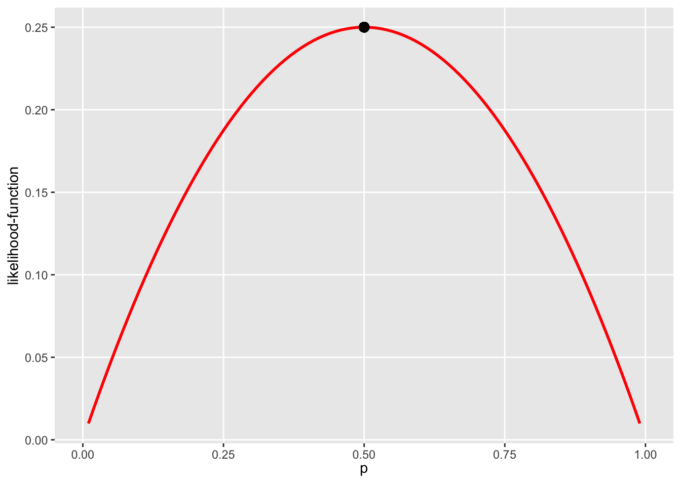
Our maximum likelihood estimate of \(p_0\) is therefore \(\hat{p}_0^{ML}=0.5\). Maximising the logarithm of the likelihood function (instead of the likelihood function itself) gives the same end-result:
library(ggplot2)
# Graph the log-likelihood function using ggplot2:
p <- seq(from=0.01, to=0.99, by=0.01)
loglik <- log(p-p^2)
plotdata <- data.frame(cbind(p, loglik))
plotdata[1:5,]
## p loglik
## 1 0.01 -4.615221
## 2 0.02 -3.932226
## 3 0.03 -3.537017
## 4 0.04 -3.259698
## 5 0.05 -3.047026graph_loglik <- ggplot(data = plotdata) +
scale_y_continuous(name = "Log-likelihood function") +
scale_x_continuous(limits = c(0, 1),
breaks = c(0, 0.25, 0.5, 0.75, 1),
name = expression(p)) +
theme(panel.grid.minor = element_blank()) +
geom_line(aes(x = p, y = loglik),
color = "red", size = 1) +
geom_point(x = 0.5, y = log(0.5^2), color = "black", size = 3)
graph_loglik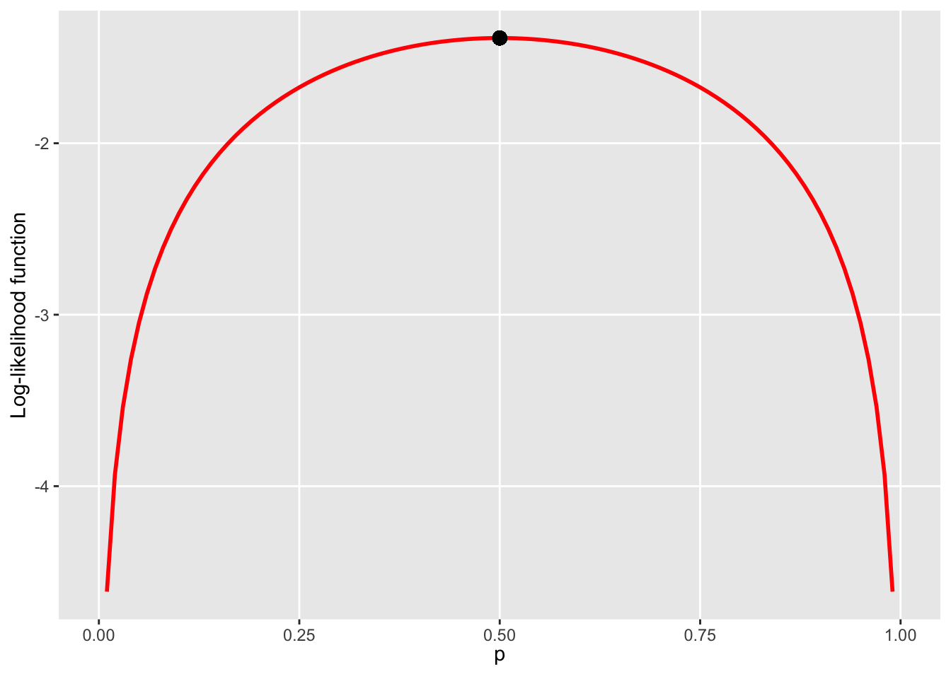
Using the log-likelihood function usually leads to simpler algebra. These ideas are generalised to deal with estimating more than one parameter as follows:
The Maximum Likelihood estimator(s) can be obtained as follows:
Let \(L_n(\theta_1,\ldots \theta_L)\) denote the Likelihood function for the whole sample of size \(n\) and let \(l_n(\theta_1,\ldots \theta_L)\) denote the log-likelihood function.
step 1: Write down the population distribution pdf \(f_X(x;\theta_1,\ldots \theta_L)\).
step 2: Derive the log-likelihood function \(l_n(\theta_1,\ldots \theta_L)\).
step 3: Solve the following system of \(L\) equations in \(L\) unknowns for \(\theta_1,\ldots \theta_L\):
\[ \frac{\delta l_n(\theta_1,\ldots \theta_L)}{\delta \theta_k} = 0 \mbox{ for } k=1,\ldots L. \]
Note that, in order to obtain the Maximum Likelihood estimator, we needed to obtain the log-likelihood function, which is a function of \(\theta\). This \(\theta\) can take any value allowed by the family of population distributions. The true population distribution, however, has one particular value of \(\theta\), the so-called true value of \(\theta\). To avoid confusion, we could have decide to denote the true value by \(\theta_0\). We will only do this in the section about the RSD of Maximum Likelihood estimators.
The easiest way to clarify the method of maximum likelihood is to apply the method to some examples.
2.1 Example 6: \(X \sim Bernoulli(p)\)
We are considering the situation where we are willing to assume that the population distribution is a member of the family of Bernoulli distributions. We are interested in finding an estimator for the parameter \(p\). We apply the method of Maximum Likelihood:
step 1: The probability mass function for the Bernoulli(\(p\)) distribution is:
\[\begin{align} f_X(x) &= P(X=x) \\ &= \begin{cases} p \;\;\;\;\;\;\; \mbox{ if } x=1 \\ 1 - p \; \mbox{ if } x=0 \end{cases} \\ &= p^x (1-p)^{1-x} \;\;\; x=0,1. \end{align}\]
step 2: Derive the log-likelihood function for \(n\) observations:
The Likelihood function for observation \(i\) is equal to:
\[ L_i(p) = p^{x_i} (1-p)^{1-x_i} \;\;\; x_i=0,1. \]
In practice, we would know the value of \(x_i\). That’s why the likelihood function is a function only of \(p\), not \(x_i\). Because we now want to derive the likelihood function for any sample of size \(n\) from the Bernoulli distribution, we do not fill in particular values and just call the value that we would obtain in practice \(x_i\). The likelihood function for the \(i^{th}\) observation just states the following obviuous fact: if \(x_i=1\), the likelihood (or: probability) of observing \(x_i\) is equal to \(p\). if \(x_i=0\), the likelihood of observing \(x_i\) is equal to \((1-p)\).
- Note that \(L_i(p)\) is just the probability mass function of step 1, with \(x\) replaced by \(x_i\). A more important difference is that \(L_i(p)\) is a function of \(p\) for a given value of \(x_i\) and \(f_X(x_i)\) is that same function viewed as a function of \(x_i\) for a given value of \(p\).
The likelihood (or: probability) of observing our whole sample is the product of the likelihoods (because of independence):
\[ L_n(p) = \Pi_{i=1}^n L_i(p) = \Pi_{i=1}^n p^{x_i} (1-p)^{1-x_i} = p^{\sum_{i=1}^n x_i}(1-p)^{n - \sum_{i=1}^n x_i}. \]
Again, we are thinking of the \(x_i\)’s as known numbers. The maximum likelihood estimator of \(p\) is the value of \(p\) that maximises this function of \(p\). As taking the derivative of the likelihood function is often quite difficult, we can use the following result:
- The argument that maximises \(l_n(p) \equiv log(L_n(p))\) is the same as the argument that maximises \(L_n(p)\). The reason is that logarithm is a strictly increasing function.
We obtain the log-likelihood function:
\[ l_n(p) = log(L_n(p)) = \sum_{i=1}^n x_i \; log(p) + (n - \sum_{i=1}^n x_i) \; log(1-p). \]
Note that we could also have derived \(l_n(p)\) in another way:
- \(L_i(p) = p^{x_i} (1-p)^{1-x_i}\).
- \(l_i(p) = log(L_i(p)) = x_i \;log(p) + (1-x_i)\;log(1-p)\).
- \(l_n(p) = \sum_{i=1}^n l_i(p) = \sum_{i=1}^n x_i \; log(p) + (n - \sum_{i=1}^n x_i) \;log(1-p)\).
step 3: Equate the first derivative of \(l_n(p)\) to zero:
\[\begin{align} \frac{d l_n(p)}{d p} &= \frac{\sum_{i=1}^n x_i}{p} - \frac{n - \sum_{i=1}^n x_i}{1-p} \\ &= \frac{(1-p) \sum_{i=1}^n x_i - p(n - \sum_{i=1}^n x_i)}{p(1-p)} \\ &= \frac{\sum_{i=1}^n x_i - pn}{p(1-p)}. \end{align}\]
As \(0<p<1\), the denominator is always positive. The first derivative can only be zero if the numerator is zero:
\[\begin{align} \frac{d l_n(p)}{d p} &= 0 \iff \\ \sum_{i=1}^n x_i - pn &= 0 \iff \\ p &= \frac{1}{n} \sum_{i=1}^n x_i. \end{align}\]
We can conclude that \(\hat{p}^{ML}= \bar{X}\).
- Note that we know, from the chapter about repeated sampling distributions, that \(Var[RSD(\hat{p}^{ML})]=\frac{p(1-p)}{n}\).
- Note that the CLT states that \(\hat{p}_{ML} \overset{approx}{\sim} N\left(p, \frac{p(1-p)}{n} \right)\) (hence \(\hat{p}_{ML}\) is consistent). This implies that \(\sum_{i=1}^n X_i \overset{approx}{\sim} N(np,np(1-p)).\)
- Note that we can give exact answers to questions about \(RSD(\hat{p}_{ML})\) using the fact that the sum of independent Bernoulli’s are Binomial (i.e. using \(\sum_{i=1}^n X_i \sim Bin(n, p)\)).
2.2 Example 7: \(X \sim Poisson(\lambda)\)
We are considering the situation where we are willing to assume that the population distribution is a member of the family of Poisson distributions. We are interested in finding an estimator for the unknown parameter \(\lambda\). We apply the method of Maximum Likelihood:
step 1: The probability mass function for the Poisson(\(\lambda\)) distribution is:
\[ f_X(x) = e^{- \lambda}\frac{\lambda^x}{x!}. \]
step 2: Derive the log-likelihood function for \(n\) observations:
The Likelihood function for observation \(i\) is equal to:
\[ L_i(p) = e^{- \lambda}\frac{\lambda^{x_i}}{x_i!}. \]
The log-Likelihood function for observation \(i\) is equal to:
\[ l_i(p) = - \lambda + x_i log(\lambda) - log(x_i!). \]
The log-Likelihood function for \(n\) observations \(l_n(\lambda)\) is equal to:
\[ l_n(\lambda) = \sum_{i=1}^n l_i(\lambda) = -n\lambda + \left( \sum_{i=1}^n x_i \right) log(\lambda) - \sum_{i=1}^n log(x_i!). \]
step 3: Equate the first derivative of \(l_n(p)\) to zero and solve:
\[\begin{align} \frac{d l_n(\lambda)}{d \lambda} &= -n + \frac{\sum_{i=1}^n x_i}{\lambda} = 0 \iff \\ \frac{1}{\lambda} &= \frac{1}{\bar{X}} \iff \\ \lambda &= \bar{X}. \end{align}\]
We can conclude that \(\hat{\lambda}^{ML}= \bar{X}=\hat{\lambda}^{MM}\). We have already shown that \(\hat{\lambda}^{MM}\) is consistent.
2.3 Example 8: \(X \sim Uniform(a,b)\)
We are considering the situation where we are willing to assume that the population distribution is a member of the family of Continuous Uniform distributions with boundaries \(a\) and \(b\). We are interested in finding an estimator for the unknown parameters \(a\) and \(b\). We apply the method of Maximum Likelihood:
step 1: The probability density function for the Uniform(\(a,b\)) distribution is:
\[ f_X(x) = \frac{1}{b-a} \;\;\;\; a<b, \; a<x<b. \]
The Likelihood function for observation \(i\) is equal to:
\[ L_i(a,b) = \frac{1}{b-a} \;\;\;\; a<b, \; a<x<b. \]
Note that this function has no maximum for finite \(a\) and \(b\): the function is infinity for \(b-a \rightarrow 0\). We will continue, but just to see where we end up. The log-Likelihood function for observation \(i\) is equal to:
\[ l_i(a,b) = - log(b-a). \]
The log-Likelihood function for \(n\) observations \(l_n(a,b)\) is equal to:
\[ l_n(a,b) = -n \; log(b-a). \]
step 3: Equate the first derivatives of \(l_n(a,b)\) to zero and solve:
\[\begin{align} \frac{d l_n(a,b)}{d a} &= \frac{n}{b-a} = 0. \\ \frac{d l_n(a,b)}{d b} &=\frac{-n}{b-a} = 0. \end{align}\]
No solution exists with both \(a\) and \(b\) finite.
So what went wrong? The boundaries of the support (the set of values for which the pdf is positive) of the density of the Continuous Uniform distribution depends on the parameters \(a\) and \(b\). In this case, the maximum likelihood method cannot be used.
2.4 Example 9: \(X \sim Normal(\mu,\sigma^2)\)
We are considering the situation where we are willing to assume that the population distribution is a member of the family of Normal distributions. We are interested in finding an estimator for the unknown parameters \(\mu\) and \(\sigma^2\). We apply the method of Maximum Likelihood:
step 1: The probability density function for the N(\(\mu,\sigma^2\)) distribution is:
\[ f_X(x) = \frac{1}{\sigma \sqrt{2 \pi}} e^{\frac{1}{2 \sigma^2}(x-\mu)^2} = (\sigma^2)^{-\frac{1}{2}} (2 \pi)^{-\frac{1}{2}} e^{-\frac{1}{2 \sigma^2}(x-\mu)^2}. \]
step 2: Derive the log-likelihood function for \(n\) observations:
The Likelihood function for observation \(i\) is equal to:
\[ L_i(\mu,\sigma^2) = (\sigma^2)^{-\frac{1}{2}} (2 \pi)^{-\frac{1}{2}} e^{-\frac{1}{2 \sigma^2}(x_i-\mu)^2} \;\;\;\; \sigma^2>0. \]
The log-Likelihood function for observation \(i\) is equal to:
\[ l_i(\mu,\sigma^2) = -\frac{1}{2} log(\sigma^2) -\frac{1}{2} log(2 \pi) - \frac{1}{2 \sigma^2}(x_i-\mu)^2. \]
The log-Likelihood function for \(n\) observations \(l_n(\mu,\sigma^2)\) is equal to:
\[ l_n(\mu,\sigma^2) = -\frac{n}{2} log(\sigma^2) -\frac{n}{2} log(2 \pi) - \frac{1}{2 \sigma^2} \sum_{i=1}^n (x_i-\mu)^2. \]
step 3: Equate the first derivatives of \(l_n(\mu, \sigma^2)\) to zero and solve:
For the derivative we will replace \(\sigma^2\) by \(\gamma\), just to not get confused with the square in \(\sigma^2\):
\[ l_n(\mu,\gamma) = -\frac{n}{2} log(\gamma) -\frac{n}{2} log(2 \pi) - \frac{1}{2 \gamma} \sum_{i=1}^n (x_i-\mu)^2. \]
\[\begin{align} \frac{\delta l_n(\mu,\gamma)}{d \mu} &= \frac{1}{\gamma} \sum_{i=1}^n (x_i-\mu) = 0. \\ \frac{\delta l_n(\mu, \gamma)}{d \gamma} &= - \frac{n}{2 \gamma} + \frac{1}{2 \gamma^2} \sum_{i=1}^n (x_i-\mu)^2 = 0. \end{align}\]
As \(\gamma > 0\), the first equation simplifies to
\[ \sum_{i=1}^n (x_i - \mu) = 0 \iff \sum_{i=1}^n x_i - n\mu = 0 \iff \mu = \frac{1}{n}\sum_{i=1}^n x_i = \bar{x}. \]
We can conlude that \(\hat{\mu}^{ML} = \bar{X}\) (which is consistent).
Substituting this result in the second equation gives:
\[ \frac{1}{2 \gamma^2} \sum_{i=1}^n (x_i-\bar{x})^2 = \frac{n}{2 \gamma}, \]
which implies that
\[ \sum_{i=1}^n (x_i - \bar{x})^2 = \gamma n \iff \gamma = \frac{1}{n} \sum_{i=1}^n (x_i - \bar{x})^2. \]
We can therefore conclude that \(\hat{\sigma}^2_{ML} = \hat{\gamma}^{ML} = \frac{1}{n} \sum_{i=1}^n (X_i - \bar{X})^2 =\hat{\sigma}^2_{MM}\). We have already shown that \(\hat{\sigma}^2_{MM}\) is consistent.
2.5 Example 10: \(X \sim Exponential(\lambda)\)
We are considering the situation where we are willing to assume that the population distribution is a member of the family of Exponential distributions. We are interested in finding an estimator for the unknown parameter \(\lambda\). We apply the method of Maximum Likelihood:
step 1: The probability density function for the Exponential(\(\lambda\)) distribution is:
\[ f_X(x) = \lambda e^{- \lambda x} \;\;\;\;\; x>0, \lambda>0. \]
step 2: Derive the log-likelihood function for \(n\) observations:
The Likelihood function for observation \(i\) is equal to:
\[ L_i(\lambda) = \lambda e^{- \lambda x_i} \;\;\;\;\; x>0, \lambda>0. \]
The log-Likelihood function for observation \(i\) is equal to:
\[ l_i(\lambda) = log(\lambda) - \lambda x_i. \]
The log-Likelihood function for \(n\) observations is equal to:
\[ l_n(\lambda) = n \; log(\lambda) - \lambda \sum_{i=1}^n x_i. \]
step 3: Equate the first derivative of \(l_n(p)\) to zero:
\[\begin{align} \frac{d l_n(\lambda)}{d \lambda} &= \frac{n}{\lambda} - \sum_{i=1}^n x_i = 0 \iff \\ \lambda \sum_{i=1}^n x_i &= n \iff \\ \lambda &= \frac{1}{\bar{X}}. \end{align}\]
We can conclude that \(\hat{\lambda}^{ML}= \frac{1}{\bar{X}} = \hat{\lambda}^{MM}\). We have already shown consistency of \(\hat{\lambda}^{MM}\) using the Delta Method.
2.6 Invariance of ML to Nonlinear Transformations of the Parameter
Some question of interest are not directly questions about the parameter of the population distribution. For example, suppose that we assume that \(X \sim Poisson(\lambda)\) and that we want to estimate the probability that \(X=x\) for \(x=3\) (if we were to estimate \(P(X=x)\) for all values of \(x\), we would be estimating the whole population distribution).
\[ P(X=3)=e^{-\lambda} \frac{\lambda^3}{3!} = e^{-\lambda} \frac{\lambda^3}{6}. \] Estimating this function of \(\lambda\) is not the same as estimating \(\lambda\) itself. When we use the maximum likelihood estimator of \(\lambda\), however, we can use the following result:
The Maximum Likelihood estimator is invariant to nonlinear transformations of the parameter:
Let \(\hat{\theta}^{ML}\) denote the maximum likelihood estimator of the (unknown) parameter of the population distribution \(\theta\). Suppose that we want to estimate some (possibly nonlinear) function of this parameter \(f(\theta)\) (instead of \(\theta\) itself).
The maximum likelihood estimator of \(f(\theta)\) is equal to:
\[ \widehat{f(\theta)}^{ML} = f(\hat{\theta}^{ML}). \]The maximum Likelihood estimator for \(P(X=3)\) is therefore:
\[ \widehat{P(X=3)}^{ML} = \widehat{e^{-\lambda} \frac{\lambda^3}{6}}^{ML}=e^{-\hat{\lambda}^{ML}} \frac{(\hat{\lambda}^{ML})^3}{6}. \]
No such invariance result holds for the Method of Moments estimator.
- Note: if you are really interested in \(P(X=3)\), you would want the RSD of \(P(X=3)\) instead of the RSD of \(\hat{\lambda}\). Obtaining this RSD is beyond the scope of this course. The required result is a theorem that is called The Delta Method. This theorem states that the RSD of \(f(\hat{\theta})\) is approximately Normal with mean \(f(\theta)\) and variance \(\{ f^{\prime}(\theta) \}^2 Var(\hat{\theta})\), where \(f^{\prime}(\cdot)\) denotes the first derivative of \(f(\cdot)\). For example, if \(f(t)=2t\), a linear function, then \(Var[2\hat{\theta}]=4 Var[\hat{\theta}]\), as expected.
2.7 The RSD of Maximum Likelihood Estimators
Let \(T_1\) and \(T_2\) be two estimators of some parameter \(\theta_0\). In this section, we will denote the true value of the unknown parameter of the population distribution by \(\theta_0\), as opposed to the argument of the log-likelihood function, which is denoted by \(\theta\). Suppose also that the two estimators are unbiased: \(E[T_1]=\theta_0\) and \(E[T_2]=\theta_0\). The estimator \(T_1\) is called more efficient than \(T_2\) if
\[ Var[T_1] < Var[T_2] \text{ for all possible values of }\theta_0. \]
Ideally, we would estimate \(\theta_0\) by using an estimator that is at least as efficient as any other estimator. It can be shown that, in large samples, the Maximum Likelihood estimator is the most efficient estimator. We will not prove this result, but the proof is based on the following observation:
Cramer-Rao lower bound for the variance of unbiased estimators:
Let \(X_1,\ldots,X_n\) be a random sample from a population with pdf \(f_X(x;\theta_0)\) and let \(T(X_1,\ldots,X_n)\) be an unbiased estimator of \(\theta_0\). Then,
\[ Var[T] \geq \frac{1}{I_n(\theta_0)}, \]
where
\[ I_n(\theta) = - E\left[ \frac{d^2 l_n(\theta)}{d \theta^2} \right]. \]
The value of \(I_n(\theta_0)\) is called the Information for n observations evaluated at the true value \(\theta_0\). The information for \(n\) observations is a function of \(\theta\): minus the expected value of the second derivative of the log-likelihood function for \(n\) observations.
Note that \(I_n(\theta) = nI_i(\theta)\), where \(I_i(\theta)\) denotes the information for observation \(i\) (minus the expected value of the second derivative of the log-likelihood function for observation \(i\)).It can be shown that the Maximum Likelihood estimator reaches this lower bound for the variance:
\[ \hat{\theta}_0^{ML} \overset{approx}{\sim} N \left( \theta_0, \frac{1}{I_n(\theta_0)} \right). \]
In practice, this result tells us three things:
- The RSD of Maximum Likelihood estimators is approximately Normal.
- The mean of the approximate RSD is equal to the true value \(\theta_0\).
- We can obtain the variance of the RSD by calculating the Information.
To obtain the Information, we should first calculate the second derivative of the log-likelihood function for \(n\) observations \(l_n(\theta)\). In order to obtain \(\hat{\theta}^{ML}\), we have already calculated the first derivative.
As a first example, consider the Exponential(\(\lambda_0\)) population distribution example.
We obtained
\[ l_n(\lambda) = n \; log(\lambda) - \lambda \sum_{i=1}^n x_i. \]
We found that \(\hat{\lambda}_0^{ML}=\frac{1}{\bar{X}}\) using the first derivative:
\[ \frac{d l_n(\lambda)}{d \lambda} = \frac{n}{\lambda} - \sum_{i=1}^n x_i. \]
The second derivative is equal to:
\[ \frac{d^2 l_n(\lambda)}{d \lambda^2} = - \frac{n}{\lambda^2}. \]
The expected value is the same, as the expression does not depend on any \(x_i\) (if it would have, we would have used \(E[X_i]=\frac{1}{\lambda_0}\)):
\[ I_n(\lambda) = - E \left[ \frac{d^2 l_n(\lambda)}{d \lambda^2} \right] = \frac{n}{\lambda^2}. \]
Evaluating the Information in the true value \(\lambda = \lambda_0\), we obtain
\[ I_n(\lambda_0) = - \left( E \left[ \frac{d^2 l_n(\lambda)}{d \lambda^2} \right] \right)_{\lambda = \lambda_0} = \frac{n}{\lambda_0^2}. \]
We can conclude the following:
\[ \hat{\lambda}_0^{ML} \overset{approx}{\sim} N \left( \lambda_0, \frac{\lambda_0^2}{n} \right). \]
This result corresponds to the result we obtained earlier: we noted that \(\hat{\lambda}_0^{ML}=\hat{\lambda}_0^{MM}\), and obtained the RSD of \(\hat{\lambda}_0^{MM}\) using the Delta Method. We can now obtain the approximate RSD of any Maximum Likelihood estimator without requiring results obtained for Method of Moment estimators.
As a second example, consider the Poisson(\(\lambda\)) population distribution.
We obtained that \(\hat{\lambda}_0^{ML}=\bar{X}\) using
\[ \frac{d l_n(\lambda)}{d \lambda} = -n + \frac{\sum_{i=1}^n x_i}{\lambda}. \] The second derivative is equal to
\[ \frac{d^2 l_n(\lambda)}{d \lambda^2} = - \frac{\sum_{i=1}^n x_i}{\lambda^2}. \] Taking the expected value (using \(E[X_i]=\lambda_0\)), we obtain
\[ E \left[ \frac{d^2 l_n(\lambda)}{d \lambda^2} \right] = - \frac{n\lambda_0}{\lambda^2}. \] Evaluating in \(\lambda = \lambda_0\) gives:
\[ \left( E \left[ \frac{d^2 l_n(\lambda)}{d \lambda^2} \right] \right)_{\lambda = \lambda_0} = - \frac{n\lambda_0}{\lambda_0^2} = - \frac{n}{\lambda_0}. \] The Information evaluated in the true value is hence \[ I_n(\lambda_0) = - \left( E \left[ \frac{d^2 l_n(\lambda)}{d \lambda^2} \right] \right)_{\lambda = \lambda_0} = \frac{n}{\lambda_0}, \]
so that
\[ \hat{\lambda}_0^{ML} \overset{approx}{\sim} N\left( \lambda_0, \frac{\lambda_0}{n} \right), \]
as expected.
As a third example, we consider the Bernoulli(\(p_0\)) population distribution.
We have found that \(\hat{p}_0^{ML}=\bar{X}\), and that
\[ \frac{d l_n(p)}{d p} = \frac{\sum_{i=1}^n x_i}{p} - \frac{n - \sum_{i=1}^n x_i}{1-p}. \]
The second derivative is
\[\begin{align} \frac{d^2 l_n(p)}{d p^2} &= -\frac{\sum_{i=1}^n x_i}{p^2} - \frac{n - \sum_{i=1}^n x_i}{(1-p)^2} \\ &= \frac{-(1-p)^2 \sum_{i=1}^n x_i - np^2 + p^2 \sum_{i=1}^n x_i }{p^2 (1-p)^2} \\ &= \frac{- \sum_{i=1}^n x_i + 2p \sum_{i=1}^n x_i - p^2 \sum_{i=1}^n x_i -np^2 + p^2 \sum_{i=1}^n x_i}{p^2 (1-p)^2} \\ &= \frac{- \sum_{i=1}^n x_i + 2p \sum_{i=1}^n x_i -n p^2}{p^2 (1-p)^2}. \end{align}\]
The expected value is (using \(E[X_i]=p_0\)):
\[ E \left[ \frac{d^2 l_n(p)}{d p^2} \right] = \frac{- n p_0 + 2n p_0 p - n p^2 }{p^2(1-p)^2}. \]
Evaluate in the true value \(p=p_0\):
\[\begin{align} \left( E \left[ \frac{d^2 l_n(p)}{d p^2} \right] \right)_{p=p_0} &= \frac{- n p_0 + 2n p_0^2 -n p_0^2}{p_0^2(1-p_0)^2} \\ &= \frac{- np_0 + np_0^2}{p_0^2 (1-p_0)^2} \\ &= \frac{-(np_0(1-p_0))}{p_0^2 (1-p_0)^2} \\ &= -\frac{n}{p_0(1-p_0)}. \end{align}\]
Hence, the Information evaluated in the true value is
\[ I_n(p_0) = - \left( E \left[ \frac{d^2 l_n(p)}{d p^2} \right] \right)_{p=p_0}= \frac{n}{p_0(1-p_0)}, \] so that
\[ \hat{p}_0^{ML} \overset{approx}{\sim} N \left( p_0, \frac{p_0(1-p_0)}{n} \right), \] as expected.
2.8 Maximum Likelihood Estimation in More Complicated Examples
We have been able to apply the maximum likelihood method to most of our examples by doing the following:
- Write down the log-likelihood function for \(n\) observations \(l_n(\theta_1,\ldots,\theta_k)\).
- Take first derivatives and equate to zero.
- Solve for the parameters.
In practice, steps 2 and 3 are often too complicated. As a result, we cannot obtain an explicit formula for the maximum likelihood estimator so that we cannot simply fill in the values observed in our particular dataset to obtain estimates.
What we can do is ask R to do step 2 and 3 for us using our particular dataset. The maxLik package contains the function maxLik that gives us the ML estimates and standard-errors. It does require us to do step 1: a log-likelihood function must be provided.
Suppose that step 1 yields the following log-liklihood:
\[ l_n(\beta_1,\beta_2)=\sum_{i=1}^n \left\{ y_i log(\Phi(\beta_1 + \beta_2 x_i)) + (1-y_i)log(1-\Phi(\beta_1+\beta_2 x_i)) \right\}. \] The variable \(y_i\) takes the values 0 or 1 and \(x_i\) is continuous. We can take the first derivative and equate to zero. Solving for \(\beta_1\) and \(\beta_2\) is too complicated.
We use logLik instead. We first generate a dataset with 100 observations on the variables y and x:
x <- rnorm(100)
beta1 <- 1
beta2 <- 2
ystar <- beta1 + beta2 * x + rnorm(100)
y <- (ystar > 0)
data <- cbind(y,x)
data[1:5,]
## y x
## [1,] 0 -1.05869741
## [2,] 1 -0.05354373
## [3,] 0 -0.24789022
## [4,] 0 -0.77413844
## [5,] 1 1.48472817The maxLik function requires us to supply the log-likelihood function for \(n\) obervations. The parameters are beta1 and beta2 (supplied in a single vector beta with two elements):
loglik <- function(beta) {
  sum( y*log(pnorm(beta[1] + beta[2]*x)) + (1-y)*log(1 - pnorm(beta[1] + beta[2]*x)) )
}
All we have to do now is provide the numerical maximisation algorithm (we use BFGS) with a starting value. The rest is taken care of by the maxLik function:
library(maxLik)
# starting values with names (a named vector)
start = c(1,1)
names(start) = c("beta1","beta2")
mle_res <- maxLik( logLik = loglik, start = start, method="BFGS" )
summary(mle_res)
## --------------------------------------------
## Maximum Likelihood estimation
## BFGS maximization, 29 iterations
## Return code 0: successful convergence
## Log-Likelihood: -29.60837
## 2 free parameters
## Estimates:
## Estimate Std. error t value Pr(> t)
## beta1 0.8892 0.2285 3.892 9.95e-05 ***
## beta2 1.8416 0.3572 5.155 2.53e-07 ***
## ---
## Signif. codes: 0 '***' 0.001 '**' 0.01 '*' 0.05 '.' 0.1 ' ' 1
## --------------------------------------------