1 Population Distribution versus Repeated Sampling Distribution

What is inferential statistics all about?

The goal of inferential statistics is:
To give a credible answer to an interesting question using data. Moreover, the uncertainty that is due to sampling should be quantified.

Let’s look at an example: consider the population distribution of incomes of people living in Portugal. For the moment, we will not assume anything about this unknown distribution. What we want is to estimate the expected value (or: mean \(\mu = E[X]\)) of this distribution. We decide to use the sample average \(\bar{X}=\frac{1}{n}\sum_{i=1}^n X_i\) as an estimator for \(E[X]\). Using a sample of size \(n=3\), we obtain \(\bar{X}=6\). How accurate is this number as an estimate of \(\mu\)?

The reason why we have to ask ourselves this question is that we know that if we were to draw another random sample of size 3 we would obtain a different value for the sample average and hence a different estimate for the unknown value of \(\mu\). Will this estimate be close to \(6\) or completely different? As it stands, we do not know. How can we quantify this uncertainty due to sampling? We will use the so-called repeated sampling distribution (RSD) of \(\bar{X}\):

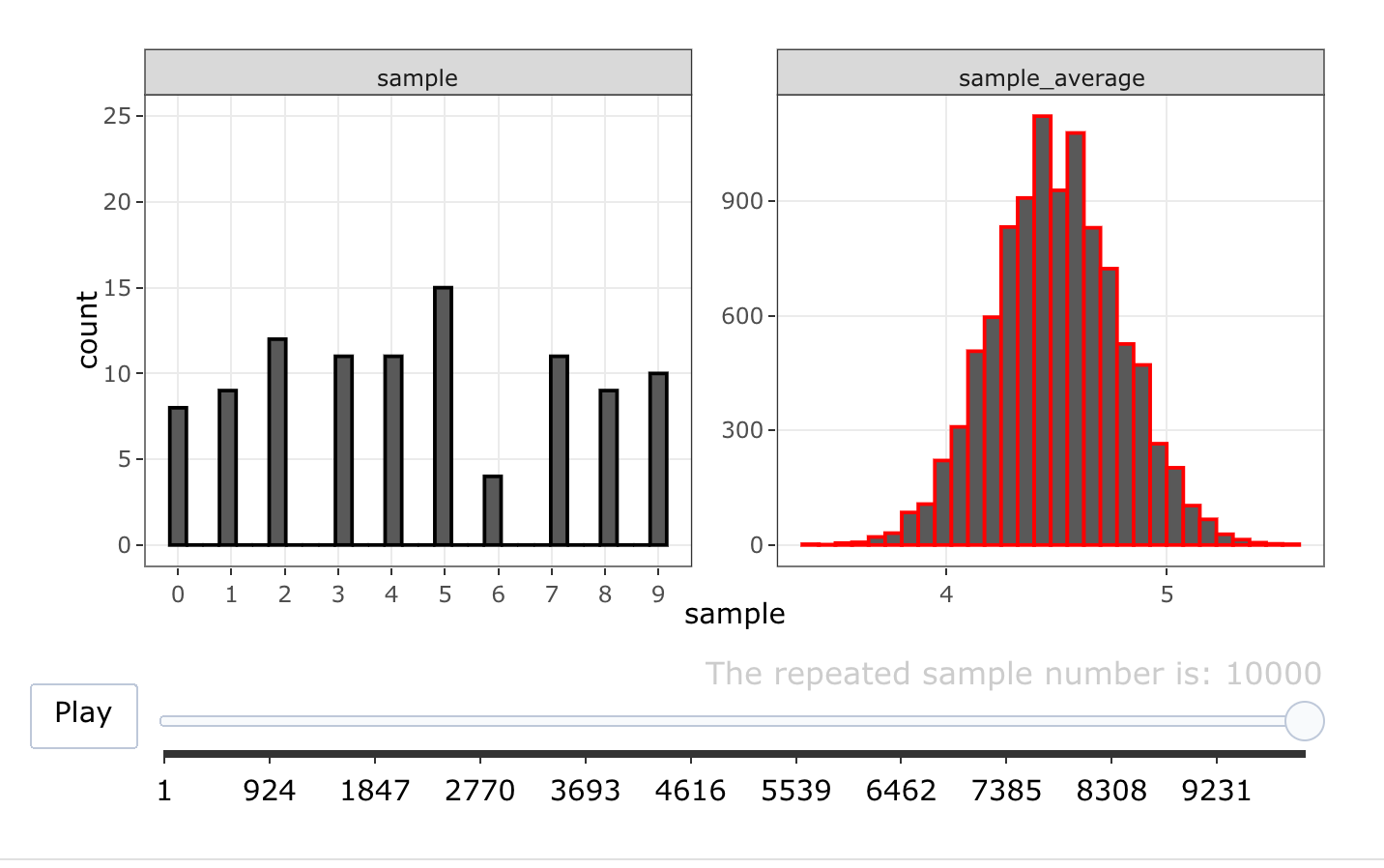
Imagine that we would obtain 10 million (or even better: infinitely many) random samples of size \(n=3\) from the income distribution. For each of those random samples, we could then obtain the sample average. The distribution of sample averages (we can plot this distribution using a histogram) is called the repeated sampling distribution of the sample average (\(RSD(\bar{X}\))). This distribution is useful for the following reason: our observed sample average \(\bar{X}=6\) can be considered a (single) draw from this distribution, i.e. we have observed a sample of size 1 from \(RSD(\bar{X})\). If the variance of \(RSD(\bar{X})\) is small, we would know that if we were to draw a second random sample of size 3, the value of the sample average that we would obtain (also a sample of size 1 from \(RSD(\bar{X})\)) will be close to 6. This means that the sampling error can be considered small if \(\mathbf{Var[RSD(\bar{X})]}\) is small!

The following animation shows what \(RSD(\bar{X})\) would look like when the population distribution is discrete uniform (which takes values between 0 and 9 with equal probability) and \(n=3\). To keep the animation short, we only draw 100 repeated samples, not 10 million:

The problem that remains is to obtain the repeated sampling distribution of \(\bar{X}\). This seems impossible, as we only have access to a single sample of size 3 and hence only have access to a single sample average (equal to 6 in our case). Fortunately, however, we can use mathematics to obtain the mean and variance of \(RSD(\bar{X})\). The mathematics required is not very complicated: three rules for the mean of a random variable and three rules for the variance of a random variable.

Using the rules, we obtain:

The first result shows that the sample average is an unbiased estimator of the population mean: in repeated samples, the sample average would on average in repeated samples estimate the value of \(E[X]\) correctly. This means that \(\bar{X}\) does not systematically over-estimate of under-estimate \(E[X]\) in repeated samples.

The second result states that the variance of the repeated sampling distribution of the sampling average equals the variance of the population distribution devided by \(n\), the sample size.

• Note that we cannot simply use the sample variance of \(RSD(\bar{X})\) to estimate \(Var[RSD(\bar{X})]\), as we only have a sample of size 1 from \(RSD(\bar{X})\). We can, however, estimate \(Var[X]\), the variance of the population distribution, using the sample variance: we have a sample of size \(n\) from the population distribution. This makes the second result very useful: we can estimate the variance of a distribution from which we have only a sample of size 1 because the second results relates this variance to the variance of a distribution from which we have a sample of size \(n\).
• Note also that we did not make any assumptions about the population distribution (e.g. we did not assume that it is a Normal distribution). Both results are true for any population distribution. We will see later that if we were to assume that the population distribution is a Normal distribution, \(RSD(\bar{X})\) will also be a Normal distribution (with mean \(E[X]\) and variance \(\frac{Var[X]}{n}\), of course).

We have been working on an example where the question was: what is the mean of a random variable \(X\) (more specifically: what is the mean income of a Portuguese person)? Other questions could be about the variance of a random variable \(X\).

Note that the variance of the population distribution can be estimated by the sample variance

\[ S^2 = \frac{1}{n}\sum_{i=1}^n (X_i - \bar{X})^2, \]

or the adjusted sample variance

\[ S^{\prime 2} = \frac{1}{n-1}\sum_{i=1}^n (X_i - \bar{X})^2. \]

The adjusted sample variance is better because it is an unbiased estimator of \(\sigma^2\):

\[ E[RSD(S^{\prime 2})] = E[S^{\prime 2}]=\sigma^2. \]

This implies that \(S^2\) is a biased estimator of \(\sigma^2\):

\[ E[RSD(S^2)]=E[S^2]=E\left[ \frac{n-1}{n}S^{\prime 2}\right]=\frac{n-1}{n}E[S^{\prime 2}]=\frac{n-1}{n}\sigma^2 \neq \sigma^2. \]

Sometimes we are more interested in the difference between the means/variances of two different populations (for instance Portugal and England). The answer to all the questions mentioned above will depend on what we assume about the population distribution (e.g. is it Normal or Exponential or Poisson?). In what follows, we will discuss several example situations and discuss the results that are required to answer (potentially interesting) questions in those situations.

Most of these questions can be answered by knowing something about the RSD of the sample average (sometimes it is easier to use the RSD of \(\sum_{i=1}^n X_i\)) or the RSD of the sample variance \(S^{\prime 2}= \frac{1}{n-1}\sum_{i=1}^n (X_i - \bar{X})^2\), given what is assumed about the population distribution.

In total, we will accumulate 15 results.

2 Questions About The Mean (or Proportion) of a Single Population

The 10 most important RSD-results for questions about the mean will turn out to be:

• linear combinations of Normals are Normal. This implies that \(X \sim N(\mu,\sigma^2) \implies \bar{X} \sim N(\mu, \frac{\sigma^2}{n})\)
• Central Limit Theorem (CLT): sample average is approximately Normal (regardless of the distribution of X)
• standardise Normal with known variance: standard-normal distribution
• standardise Normal with estimated variance: t distribution
• sum of Bernoulli(\(p\)) is Binomial(\(n,p\))
• Binomial(\(n,p\)) with large \(n\) and small \(p\) is approximately Poisson(\(\lambda=np\))
• sum of Poisson(\(\lambda_i\)) is Poisson(\(\sum_{i=1}^n \lambda_i\))
• constant (c) times Exponential(\(\lambda\)) is Exponential(\(\frac{\lambda}{c}\))
• sum of Exponential(\(\lambda\)) is Gamma(\(n,\lambda\))
• \(2\lambda\) times Gamma(\(n,\lambda\)) is Chi-squared(\(2n\))

# CLT approximation:
pnorm((5.5-10)/sqrt(10)) - pnorm((4.5-10)/sqrt(10))

## [1] 0.0363693

# Exact:
dpois(5, lambda=10)

## [1] 0.03783327

set.seed(1234)
rbinom(5, size=1, prob=0.25)

## [1] 0 0 0 0 1

set.seed(1234)
round( dbinom(0:10, size = 30, prob=0.1), 2)

##  [1] 0.04 0.14 0.23 0.24 0.18 0.10 0.05 0.02 0.01 0.00 0.00

round( dpois(0:10, lambda=3), 2)

##  [1] 0.05 0.15 0.22 0.22 0.17 0.10 0.05 0.02 0.01 0.00 0.00

set.seed(1234)
round( dbinom(10:20, size = 30, prob=0.5), 2)

##  [1] 0.03 0.05 0.08 0.11 0.14 0.14 0.14 0.11 0.08 0.05 0.03

round( dpois(10:20, lambda=15), 2)

##  [1] 0.05 0.07 0.08 0.10 0.10 0.10 0.10 0.08 0.07 0.06 0.04

3 Questions About The Means (or Proportions) of Two Populations

No new RSD-results are required for questions about two means

Suppose that we have two random samples. The first random sample (\(X_{11}, \ldots X_{1 n_1}\)) is a sample of incomes from Portugal and has size \(n_1\). The second random sample ((\(X_{21}, \ldots X_{2 n_2}\))) is a sample of incomes from England and has size \(n_2\). We want to compare the mean of the income distribution in Portugal with the mean of the income distribution in England. The obvious thing to do is to compare \(\bar{X}_1\), the sample average of the Portuguese sample, with \(\bar{X}_2\), the sample average of the English sample. In particular, we would compute \(\bar{X}_1 - \bar{X}_2\). What is the repeated sampling distribution of \(\bar{X}_1 - \bar{X}_2\)? The answer will depend on what we are willing to assume about the income distributions in Portugal (\(X_1\)) and England (\(X_2\)).

4 Questions About The Variance of A Single Population

The 3 most important RSD-results for questions about the variance will turn out to be:

• sum of standard-normal-squared is Chi-squared(\(n\))
• Estimate \(r\) parameters: substract \(r\) from the number of degrees of freedom
• This implies: \(\frac{(n-1)S^{\prime 2}}{\sigma^2}\) is Chi-squared(\(n-1\))

5 Questions About The Variances of Two Populations

The 2 most important RSD-results for questions about two variances will turn out to be:

• \(\frac{Chi-squared(a)/a}{Chi-squared(b)/b}\) is \(F_{a,b}\)
• This implies: \(\frac{S_1^{\prime 2} / \sigma^2_1 }{ S_2^{\prime 2} / \sigma^2_2} \sim F_{n_1-1, n_2-1}\)

Suppose that we have two random samples. The first random sample (\(X_{11}, \ldots X_{1 n_1}\)) is a sample of incomes from Portugal and has size \(n_1\). The second random sample (\(X_{21}, \ldots X_{2 n_2}\)) is a sample of incomes from England and has size \(n_2\). We want to compare the variance of the income distribution in Portugal with the variance of the income distribution in England. The obvious thing to do is to compare \(S^{\prime 2}_1\), the adjusted sample variance of the Portuguese sample, with \(S^{\prime 2}_2\), the adjusted sample variance of the English sample. In particular, we would compute \(S^{\prime 2}_1 -S^{\prime 2}_2\). Unfortunately, there is no easy way to obtain the repeated sampling distribution of \(S^{\prime 2}_1 -S^{\prime 2}_2\).

If we assume that both population distributions are Normal, we can derive a result that comes close enough.

qf(0.05, df1=10, df2=20)

## [1] 0.3604881

1 / qf(0.95, df1=20, df2=10)

## [1] 0.3604881

6 Questions about the Maximum or Minimum (Order Statistics)

Consider a random sample of size \(n\): \(X_1,X_2, \ldots ,X_n\). If we were to sort the sample in ascending order, we obtain the so-called order statistics \(X_{(1)}, X_{(2)}, \ldots , X_{(n)}\). Hence, the minimum value that will be obtained in the sample is denoted by \(X_{(1)}\) and the maximum value that will be obtained in the sample is denoted by \(X_{(n)}\).

Sometimes we are more interested in the repeated sampling distribution of the maximum value that occurs in a sample than in the population mean or the population variance. For instance, if we build a dike to protect us from possibly rising sea-levels due to global warming, we are interested in the probability that the maximum sea-level in a sample of \(n\) months is larger than the heigth of the dike. This is an interesting question because, if this probability is high, we are likely to all drown.

We can link the cumulative distribution function of the RSD of the maximum value in the sample (\(F_{X_{(n)}}(x)\)) with the cumulative distribution of the population distribution (\(F_X(x)\)) by noting the following: the maximum value obtained in the sample is smaller than \(x\) if all values in the sample are smaller than \(x\):

\[\begin{align} F_{X_{(n)}}(x) &= P(X_{(n)} < x) \\ &= P(X_1<x, \ldots, X_n < x) \\ &\overset{ind.}{=} P(X_1<x)P(X_2<x) \cdots P(X_n<x) \\ &\overset{id.}{=} \{P(X<x)\}^n \\ &= \{F_X(x)\}^n. \end{align}\]

Suppose that the dikes are 15 meters high and we measure the sea level monthly for a year. If sea-levels follow an Exponential distribution with \(\lambda=0.1\), then \(P(X_{(12)} < 15) = \{ 1 - e^{-0.1*15}\}^{12}=0.048\), about \(5\%\). The dikes are (almost certainly) too low.

In other cases, we are more interested in the repeated sampling distribution of the minimum value obtained in a sample of size \(n\) (for instance, if you sell oxygen bottles to a group of \(n\) rather agressive looking divers that ask you how long the oxygen will last “for sure”).

We can link the cumulative distribution function of the RSD of the minimum value in the sample (\(F_{X_{(1)}}(x)\)) with the cumulative distribution of the population distribution (\(F_X(x)\)) by noting the following: the minimum value obtained in the sample is larger than \(x\) if all values in the sample are larger than \(x\):

\[\begin{align} F_{X_{(1)}}(x) &= P(X_{(1)}<x) \\ &= 1 - P(X_{(1)}>x) \\ &= 1- P(X_1>x, \ldots ,X_n>x) \\ &\overset{ind.}{=} 1-P(X_1>x) P(X_2>x) \cdots P(X_n>x) \\ &\overset{id.}{=} 1-\{P(X>x)\}^n \\ &= 1 - \{1- F_X(x)\}^n. \end{align}\]

Suppose that there are 20 divers that end up diving for 2 hours and 20 minutes (140 minutes), following your suggestion. If the number of minutes that a bottle provides oxygen follows a Normal distribution with mean 155 minutes and variance of 100, then

\[\begin{align} P(X_{(1)} > 140) &= 1 - P(X_{(1)} < 140) \\ &= 1 - ( 1 - \{1- F_X(140)\}^{20}) \\ &= \left\{ 1- F_X(140) \right\}^{20} \\ &= \left\{ 1 - P \left( \frac{X - 155}{\sqrt{100}} < \frac{140 - 155}{\sqrt{100}} \right) \right\}^{20} \\ &= \{1 - \Phi(-1.5) \}^{20} \\ &= 0.25. \end{align}\]

The probability that all divers have enough oxygen is only about \(25\%\). You better run…

Note that \(P(X>140)=1-F_X(140)=1-\Phi(\frac{140-155}{10})=1-\Phi(-1.5)=0.93\). Each bottle in itself was very likely to give enough oxygen.