7. Testing Goodness-of-fit and Independence

1 Univariate Distributions
2 Bivariate Distributions

1 Univariate Distributions

We will discuss a method to test the null-hypothesis that the population distribution is some pre-specified member of the family of Multinomial distributions. For instance: somebody claims to know that $50 %$ of the people go to work by car, $10 %$ go to work by car-pooling, $20 %$ go to work by train and $20 %$ go to work by bus. This null-hypothesis can be formulated as follows:

Let $X$ be a random variable whose distribution is a member of the family of multinomial distributions with four groups ( $k = 4$ ).
The null-hypothesis is: $H_{0} : p_{1} = 0.5, p_{2} = 0.1, p_{3} = 0.2$ , $p_{4} = 0.2$ .
The alternative hypothesis is: $H_{1} : o t h e r w i s e$ .

The dataset Mode (from the Ecdat package) has $n = 453$ observations. Each person answered some questions concerning commuting to work. The variable choice is the variable we are interested in here. We show the first 10 observations of the dataset:

library(Ecdat)
data(Mode)
attach(Mode) #attach the dataset. choice is the variable we want.

library(DT)
library(widgetframe)

dt <- datatable(Mode, caption = "The Raw Data")
frameWidget(dt, height = 550) #only necessary in Hugo Academic webpages

We do not need all the $453$ observations on the variable choice: all we need to know is the number of people that are observed in each of the 4 groups. These numbers are called frequencies or counts.

Obs_counts <- table(choice)
Obs_counts

## choice
##     car carpool     bus    rail 
##     218      32      81     122

Based on these 4 numbers, should we reject the null-hypothesis?

Our data is $O_{1} = 218$ , $O_{2} = 32$ , $O_{3} = 81$ and $O_{4} = 122$ .
How many people do we expect to observe in group 1 if $H_{0}$ is true? $E_{1} = n \times p_{1} = 453 \times 0.5 = 226.5$ .
How many people do we expect to observe in group 2 if $H_{0}$ is true? $E_{2} = n \times p_{2} = 453 \times 0.1 = 45.3$ .
How many people do we expect to observe in group 3 if $H_{0}$ is true? $E_{3} = n \times p_{3} = 453 \times 0.2 = 90.6$ .
How many people do we expect to observe in group 4 if $H_{0}$ is true? $E_{4} = n \times p_{4} = 453 \times 0.2 = 90.6$ .

We can test the null-hypothesis using the Q-statistic:

$Q = k \sum i = 1 \frac{(O_{i} - E_{i})^{2}}{E_{i}} a p p r o x \sim H_{0} χ_{k - 1}^{2} .$

We reject the null-hypothesis when $Q$ is too large: in that case, the $O_{i}$ ’s are very different from the $E_{i}$ ’s, so that the numerator becomes a large positive number (we only divide by $E_{i}$ so that finding RSD(Q) is easier).

When is $Q$ large enough to reject the null-hypothesis? It can be shown that, under $H_{0}$ , the repeated sampling distribution of $Q$ is the so-called chi-squared distribution with $k - 1$ degrees of freedom. The decision-rule is therefore:

Reject the null-hypothesis when $Q_{o b s}$ is larger than $q_{0.95}^{χ_{k - 1}^{2}}$ .

We often make assumptions like the following: the population distribution is a member of the family of Poisson distributions with (unknown) parameter $λ$ . We can use the Q-statistic (or: the chi-squared test) to test this hypothesis as well:

We first estimate the unknown parameters (by Maximum Likelihood). Here we have one unknown parameter ( $λ$ ) so that $e = 1$ .
Suppose that $^λ = 2$ . We can now test the null-hypothesis that $X$ has a Poisson distribution with $λ = 2$ using the Q-statistic.
As $λ$ was estimated (instead of it being known), we have more uncertainty than before. The approximate repeated sampling distribution of the $Q$ statistic if the null hypothesis is true is now the $χ_{k - 1 - e}^{2}$ distribution: we use degrees of freedom equal to $k - 2$ instead of $k - 1$ in this example.

We can also use the chi-squared test to test null-hypotheses with continuous distributions: all we have to do is discretise the continuous distribution to obtain a multinomial distribution. We can then apply the test using the multinomial null-hypothesis. Again, if the distribution has unknown parameters, we estimate them before discretising.

Chi-squared Test: The Method (Univariate)

step 1: specify $H_{0}$ , possibly after first estimating $e$ parameters (and discretising if $X$ is continuous): a Multinomial distribution with $k$ groups.
step 2: Calculate $E_{i} = n p_{i}$ , the expected frequencies if $H_{0}$ is true, for $i = 1, \dots, k$ . For each $i$ , we need $E_{i} \geq 5$ .
step 3: Calculate $Q_{o b s} = \sum_{i = 1}^{k} \frac{(O_{i} - E_{i})^{2}}{E_{i}}$ and reject $H_{0}$ if $Q_{o b s} > q_{0.95}^{χ_{k - 1 - e}^{2}}$ .

The method is best explained by applying it to some examples. There are several types of situations to consider:

Is the distribution under the null-hypothesis (a) discrete or (b) continuous?
Is the distribution under the null-hypothesis (1) completely known or (2) does it contain unknown parameters?

This leads to four possible cases, 1a, 1b, 2a and 2b. We will discuss an example for each of those.

1.1 Case 1a: Known Discrete Distribution

apply the Chi-squared test directly with $e = 0$
Make sure that that $E_{i} \geq 5$ for $i = 1, 2, \dots, k$ .

Suppose that the null-hypothesis is $H_{0} : X \sim P o i s s o n (λ = 2)$ . It is up to the researcher (you) how many groups to use. In this example, we could define the 9 groups as “group i consists of the people with $X = i - 1$ for $i = 1, 2, \dots, 9$ ”. This occurs because $P (X = x)$ is only positive for $x = 0, 1, \dots 8$ :

round(dpois(0:10, 2), 3)

##  [1] 0.135 0.271 0.271 0.180 0.090 0.036 0.012 0.003 0.001 0.000 0.000

To be precise, we actually take group 9 to contain the people with $X \geq 8$ . This grouping is problematic for the following reason: the $E_{i}$ ’s must always be larger or equal to 5. If some $E_{i}$ ’s are smaller than 5, the RSD of Q is not well-approximated by the chi-squared distribution, it turns out (this is not obvious).

As an example, we draw a random sample of size $n = 50$ from the Poisson( $λ = 3$ ) distribution (so the null-hypothesis is false), and calculate the frequencies:

set.seed(1234)
data <- rpois(50, lambda=3)
O <- table(data)
O

## data
##  0  1  2  3  4  5  6  8 
##  3  4 16 14  7  4  1  1

These are the $0_{i}$ ’s. If the null-hypothesis is true, our expectations about the frequencies are described by the $E_{i}$ ’s. For $n = 50$ , we obtain:

E <- 50*dpois(0:10, lambda=2)
round(E, 3)

##  [1]  6.767 13.534 13.534  9.022  4.511  1.804  0.601  0.172  0.043  0.010
## [11]  0.002

As $E_{5} = 4.511 \leq 5$ , we need to reduce the number of groups to $k = 5$ . A person will be part of group 5 if $X \geq 4$ (instead of $X = 4$ ). The corresponding probability is $P (X \geq 4) = 1 - P (X \leq 3) = 0.1428$ . The new $E_{5}$ is therefore equal to $50 \times 0.1428 = 7.14 \geq 5$ .

Using the new grouping, the observed Q-statistic is equal to:

O_new <- c(O[1:4], sum(O[5:8]))
O_new

##  0  1  2  3    
##  3  4 16 14 13

E_new <- c( E[1:4], sum(E[5:11]) )
E_new

## [1]  6.766764 13.533528 13.533528  9.022352  7.143412

Q_obs <- sum( (O_new - E_new)^2/E_new )
Q_obs

## [1] 16.80984

qchisq(0.95, df=4)

## [1] 9.487729

As $Q_{o b s} = 16.81 > 9.48$ , we (correctly) reject the null-hypothesis that $λ = 2$ .

We could also have let R calculate everything for us, using the command chisq.test:

#poisson(2) null-hypothesis probabilities:
p=dpois(0:3, lambda=2)
p

## [1] 0.1353353 0.2706706 0.2706706 0.1804470

sum(p)

## [1] 0.8571235

#Chi-squared-test:
chisq.test(x=c(3, 4, 16, 14, 13), 
           p=c(p, 1-sum(p)) )

## 
##  Chi-squared test for given probabilities
## 
## data:  c(3, 4, 16, 14, 13)
## X-squared = 16.809, df = 4, p-value = 0.002105

1.2 Case 1b: Known Continuous Distribution

discretise to k categories
apply Chi-squared test with $e = 0$

Suppose that we want to test the null-hypothesis that $X \sim E x p (λ = 0.2)$ . The mean of this distribution is equal to $5$ and the variance is equal to $25$ . We make a quick plot:

x <- 0:20
prob <- dexp(x, rate=0.2)
plot(x=x, y=prob, type ="l", col="red", xlab="x", 
     ylab="Expl(0.2)", ylim=c(0,0.3))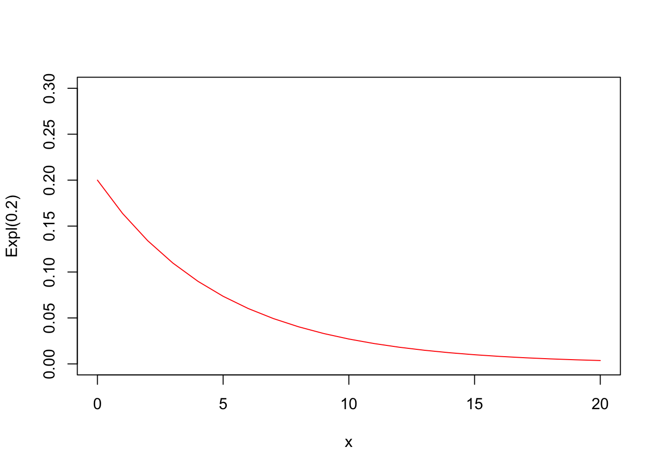

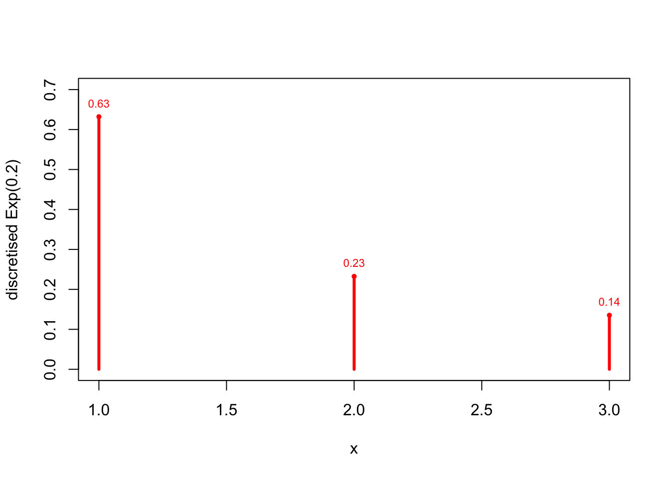
We choose to discretise with $3$ groups: $0 < X < 5$ , $5 < X < 10$ and $X > 5$ :

p_1 <- pexp(5, rate=0.2)
p_2 <- pexp(10, rate=0.2) - pexp(5, rate=0.2)
p_3 <- 1 - p_1 - p_2

x <- 1:3
prob <- c(p_1,p_2,p_3)
prob

## [1] 0.6321206 0.2325442 0.1353353

plot(x=x, y=prob, type ="h", lwd=3, col="red", xlab="x", 
     ylab="discretised Exp(0.2)", ylim=c(0,0.7))
points(x, prob, pch=16, cex=0.7, col="red")
text(x, prob, pos=3, cex=0.7, col="red", 
     labels = format(round(prob,2), nsmall=2)
     )

This will be the distribution under the null-hypothesis. As we example, we generate a random sample of $n = 100$ from the Exponential( $λ = 0.2$ ) distribution (so that the null-hypothesis is, in fact, true):

data <- rexp(100, rate=0.2)
data_discretised <- cut(data, breaks=c(0,5,10,50))
obs_counts <- table(data_discretised)
obs_counts

## data_discretised
##   (0,5]  (5,10] (10,50] 
##      71      13      16

n <- 100
E <- n*prob
E

## [1] 63.21206 23.25442 13.53353

Q <- sum((obs_counts - E)^2/E)
Q

## [1] 5.930866

# using chisq.test:
res <- chisq.test(x=obs_counts, p=prob)
res

## 
##  Chi-squared test for given probabilities
## 
## data:  obs_counts
## X-squared = 5.9309, df = 2, p-value = 0.05154

qchisq(0.95, df=2)

## [1] 5.991465

As $Q_{o b s} = 5.930866 ≯ 5.991465$ , we (correctly) do not reject the null-hypothesis.

1.3 Case 2a: Discrete Distribution with Unknown parameters

Estimate parameters
apply Chi-squared test with $e \neq 0$

As an example, we test the null-hypothesis that $X \sim P o i s s o n (λ)$ . We draw a random sample of size $n = 100$ from the Poisson( $λ = 3$ ) distribution (so the null-hypothesis is, in fact, true), and calculate the observed frequencies. We use the five groups of case 1a: $X = 0$ , $X = 1$ , $X = 2$ , $X = 3$ and $X \geq 4$ :

set.seed(1234)
data <- rpois(100, lambda=3)
data

##   [1] 1 3 3 3 5 3 0 2 4 3 4 3 2 6 2 5 2 2 1 2 2 2 1 0 2 4 3 5 5 0 3 2 2 3 1 4 2
##  [38] 2 8 4 3 3 2 3 2 3 4 3 2 4 1 2 4 3 1 3 3 4 1 5 5 0 2 0 2 4 2 3 1 3 1 5 0 4
##  [75] 1 3 2 1 2 4 6 3 1 3 1 5 2 2 1 5 1 5 1 1 1 3 2 0 2 4

O_help <- table(data)
O_help

## data
##  0  1  2  3  4  5  6  8 
##  7 18 26 23 13 10  2  1

O <- c(O_help[1:4], sum(O_help[5:8]))
O

##  0  1  2  3    
##  7 18 26 23 26

The probabilities under the null hypothesis and the expected frequencies under the null-hypothesis are:

n <- 100
lambda_hat <- mean(data)
help <- dpois(0:3, lambda=lambda_hat)
prob <- c(help, 1 - sum(help))
prob

## [1] 0.07353454 0.19192516 0.25046233 0.21790223 0.26617573

E <- n*prob
E

## [1]  7.353454 19.192516 25.046233 21.790223 26.617573

The observed Q-statistic is equal to:

Q_obs <- sum( (O - E)^2/E )
Q_obs

## [1] 0.2088999

qchisq(0.95, df=3)

## [1] 7.814728

1 - pchisq(0.2089, df=3)

## [1] 0.9761399

#using chisq.test:
chisq.test(O, p=prob)

## 
##  Chi-squared test for given probabilities
## 
## data:  O
## X-squared = 0.2089, df = 4, p-value = 0.9949

As $Q_{o b s} = 0.2088999 ≱ 7.814728$ , we (correctly) do not reject the null-hypothesis that $X \sim P o i s s o n (λ)$ . The correct p-value is equal to $0.9761399$ : the chisq.test command does not take into account that $λ$ was estimated (as it cannot know this).

1.4 Case 2b: Continuous Distribution with Unknown parameters

Estimate parameters
Discretise
apply Chi-squared test with $e \neq 0$

We use the same example as in case 1b, with null-hypothesis $H_{0} : X \sim E x p (λ)$ . We estimate $λ$ using the maximum likelihood estimator:

${^λ}_{M L} = \frac{1}{¯ X} .$

We then discretise using the three groups we used before, calculate Q and compare with $q_{0.95}^{χ_{k - 1 - e}^{2}}$ with $e = 1$ in this case:

#estimate lambda using raw data:
set.seed(12345)
raw_data <- rexp(100, rate=0.2)
lambda_hat <- 1/mean(raw_data)
lambda_hat

## [1] 0.2000546

#calculate probabilities under H0:
p_1 <- pexp(5, rate=lambda_hat)
p_2 <- pexp(10, rate=lambda_hat) - pexp(5, rate=lambda_hat)
p_3 <- 1 - p_1 - p_2

x <- 1:3
prob <- c(p_1,p_2,p_3)
prob

## [1] 0.6322210 0.2325176 0.1352614

We see that the probabilities under the null-hypothesis have not changed much. We now discretise the data, calculate the frequencies and perform the test:

# discretise the data and calculate counts:
data_discretised <- cut(raw_data, breaks=c(0,5,10,50))
obs_counts <- table(data_discretised)
obs_counts

## data_discretised
##   (0,5]  (5,10] (10,50] 
##      66      21      13

# chi-squared test:
chisq.test(obs_counts, p=prob)

## 
##  Chi-squared test for given probabilities
## 
## data:  obs_counts
## X-squared = 0.36059, df = 2, p-value = 0.835

# Correct critical value and p-value:
qchisq(0.95, df=1)

## [1] 3.841459

1 - pchisq(0.36059, df=1)

## [1] 0.5481787

As $Q_{o b s} = 0.36059 ≯ 3.841459$ , we (correctly) do not reject the null-hypothesis. The correct p-value is $0.5481787$ : the chisq.test command does not take into account that we estimated one parameter (as it cannot know this).

2 Bivariate Distributions

The distribution under the null-hypothesis is now a bivariate discrete distribution. For example, somebody could be claiming to know that the population distribution has the following probability mass function:

$f_{X, Y} (i, j) = P (X = i, Y = j) = \frac{i + j}{12} for i = 1, 2, 3 and j = 1, 2.$

The random variable $X$ has $r = 3$ categories and the random variable $Y$ has $c = 2$ categories. We can graph the $6$ probabilities of this bivariate population distribution:

We can also simply display the population probabilities in 2-by-3 table (in general this table is $r$ -by- $c$ ):

Prob	$Y = 1$	$Y = 2$	$Y = 3$	$T o t a l$
$X = 1$	$p_{11} = \frac{2}{21}$	$p_{12} = \frac{3}{21}$	$p_{13} = \frac{4}{21}$	$p_{1 ∙} = \frac{9}{21}$
$X = 2$	$p_{21} = \frac{3}{21}$	$p_{22} = \frac{4}{21}$	$p_{23} = \frac{5}{21}$	$p_{2 ∙} = \frac{12}{21}$
$T o t a l$	$p_{∙ 1} = \frac{5}{21}$	$p_{∙ 2} = \frac{7}{21}$	$p_{∙ 3} = \frac{9}{21}$	$p_{∙ ∙} = 1$

Note that we have introduced notation for the marginal distributions: the marginal probability $P (X = 1)$ , for example, is denoted by $p_{1 ∙}$ :

$P (X = 1) = 3 \sum j = 1 P (X = 1, Y = j) = 3 \sum j = 1 p_{1 j} \equiv p_{1 ∙}$

When we draw a random sample of size $n = 100$ from this population distribution, we obtain (after calculating the frequencies from the raw data):

set.seed(12345)
raw_data <- rmultinom(n=100, size=1, prob=c(2/21,3/21,3/21,4/21,4/21,5/21))
raw_data[,1:10]

##      [,1] [,2] [,3] [,4] [,5] [,6] [,7] [,8] [,9] [,10]
## [1,]    0    0    0    1    0    0    0    0    0     0
## [2,]    1    1    0    0    0    0    0    0    0     0
## [3,]    0    0    0    0    0    0    1    0    0     0
## [4,]    0    0    0    0    0    0    0    1    1     0
## [5,]    0    0    1    0    0    1    0    0    0     0
## [6,]    0    0    0    0    1    0    0    0    0     1

freq <- rowSums(raw_data)
freq

## [1] 14 12 16 18 18 22

table <- matrix(freq, nrow = 2)
table

##      [,1] [,2] [,3]
## [1,]   14   16   18
## [2,]   12   18   22

Note that when we drew a random sample from the population distribution, we just used a vector of probabilities (not a matrix of probabilities). There is no real difference between a bivariate distribution with $6$ probabilities $p_{i j}$ and a univariate distribution with $6$ probabilities $p_{i}$ . We only use the two subscripts $i$ and $j$ because it is more intuitive given that the data is organised that way. We can introduce notation for row-totals and column-totals as follows:

Freq	$Y = 1$	$Y = 2$	$Y = 3$	$T o t a l$
$X = 1$	$O_{11} = 14$	$O_{12} = 16$	$O_{13} = 18$	$O_{1 ∙} = 48$
$X = 2$	$O_{21} = 12$	$O_{22} = 18$	$O_{23} = 22$	$O_{2 ∙} = 52$
$T o t a l$	$O_{∙ 1} = 26$	$O_{∙ 2} = 34$	$O_{∙ 3} = 40$	$n = O_{∙ ∙} = 100$

With the notation for bivariate distributions (and observed frequencies) established, we can now formulate the method to test the null-hypothesis that the population distribution is some pre-specified bivariate Multinomial distribution:

Chi-squared Test: The Method (Bivariate)

step 1: specify $H_{0}$ , possibly after first estimating $e$ parameters (and discretising if $X$ is continuous): a Multinomial distribution with $k = r c$ groups.
step 2: Calculate $E_{i j} = n p_{i j}$ , the expected frequencies if $H_{0}$ is true, for $i = 1, \dots, r$ and $j = 1, \dots, c$ . For each $(i, j)$ , we need $E_{i j} \geq 5$ .
step 3: Calculate $Q_{o b s} = \sum_{i = 1}^{r} \sum_{j = 1}^{c} \frac{(O_{i j} - E_{i j})^{2}}{E_{i j}}$ and reject $H_{0}$ if $Q_{o b s} > q_{0.95}^{χ_{r c - 1 - e}^{2}}$ .

2.1 Case 3a: Known Bivariate Discrete Distributions

apply the Chi-squared test directly with $e = 0$
Make sure that that $E_{i j} \geq 5$ for $i = 1, 2, \dots, r$ and $j = 1, 2, \dots, c$ .

In the example above, the null-hypothesis was that the population distribution was a bivariate discrete distribution with known probabilities $p_{i j}$ . This example is hence of case 3a. We can simply calculate the chi-squared statistic $Q$ : there is no need to estimate parameters and there is also no need to discretise.

# Calculate Q ourselves:
n <- 100
prob=c(2/21,3/21,3/21,4/21,4/21,5/21)
sum((freq-n*prob)^2/(n*prob))

## [1] 2.928

qchisq(0.95, df=5)

## [1] 11.0705

# Check result using chisq.test:
chisq.test(x=freq, p=prob)

## 
##  Chi-squared test for given probabilities
## 
## data:  freq
## X-squared = 2.928, df = 5, p-value = 0.7111

As $Q_{o b s} = 2.928 ≯ 11.07$ , we (correctly) do not reject the null-hypothesis. The p-value is 0.7111.

2.2 Case 3b: Known Bivariate Continuous Distributions

Discretise
apply Chi-squared test with $e = 0$

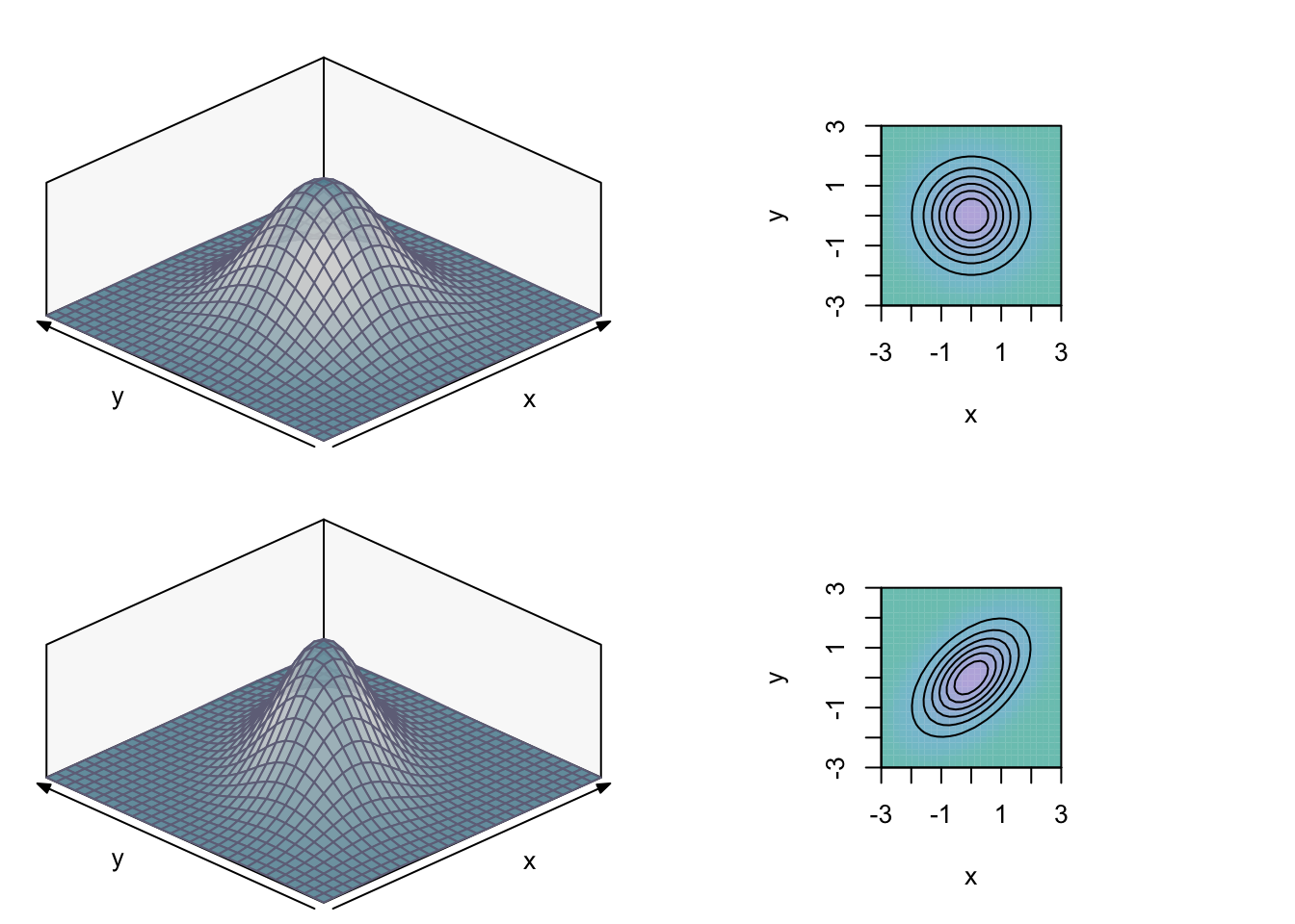
The most commonly used continuous bivariate distribution is the bivariate Normal distribution. Its marginal distributions are univariate Normals. The random variables $X$ and $Y$ can be correlated or uncorrelated (in which case they are independent). In the graph below, the marginal distributions are taken to be standard-normal. In the upper graphs, $X$ and $Y$ have $C o v [X, Y] = 0$ . The lower graphs show the bivariate density with $C o v [X, Y] = C o r r [X, Y] = 0.5$ . The graphs on the right show the distributions using isoquants (a helicopter-view), which is often easier to interpret.

We will take the uncorrelated bivariate standard Normal distribution as our null-hypothesis. As both $X$ and $Y$ take most values between $- 2$ and $2$ , we discretise the bivariate continuous distribution into $16$ areas, with both $X$ and $Y$ divided by the intervals $(- \infty, - 1)$ , $(- 1, 0)$ , $(0, 1)$ and $(1, \infty)$ . Note that, for bivariate distributions,

The pbivnorm command from the pbivnorm package can be used to calculate the values of the cdf of bivariate Normal distributions:

library(pbivnorm)
#upper-left area
p_11 <- pbivnorm(x=-1, y=10, rho=0) - pbivnorm(x=-10, y=10, rho=0) -
  pbivnorm(x=-1, y=1, rho=0) + pbivnorm(x=-10, y=-10, rho=0)
p_14 <- p_11
p_41 <- p_11
p_44 <- p_11

p_12 <- pbivnorm(x=0, y=10, rho=0) - pbivnorm(x=-1, y=10, rho=0) -
  pbivnorm(x=0, y=1, rho=0) + pbivnorm(x=-1, y=1, rho=0)
p_13 <- p_12
p_42 <- p_12
p_43 <- p_12

p_21 <- pbivnorm(x=-1, y=1, rho=0) - pbivnorm(x=-10, y=1, rho=0) -
  pbivnorm(x=-1, y=0, rho=0) + pbivnorm(x=-10, y=0, rho=0)
p_31 <- p_21
p_24 <- p_21
p_34 <- p_21

p_22 <- pbivnorm(x=0, y=1, rho=0) - pbivnorm(x=-1, y=1, rho=0) -
  pbivnorm(x=0, y=0, rho=0) + pbivnorm(x=-1, y=0, rho=0)
p_23 <- p_22
p_32 <- p_22
p_33 <- p_22

c(p_11,p_12,p_21,p_22)

## [1] 0.02517149 0.05415614 0.05415614 0.11651624

prob <- c(p_11, p_21, p_31, p_41, 
          p_12, p_22, p_32, p_42, 
          p_13, p_23, p_33, p_43, 
          p_14, p_24, p_34, p_44)
sum(prob)

## [1] 1

We can now plot the discretised version of our bivariate standard-normal distribution:

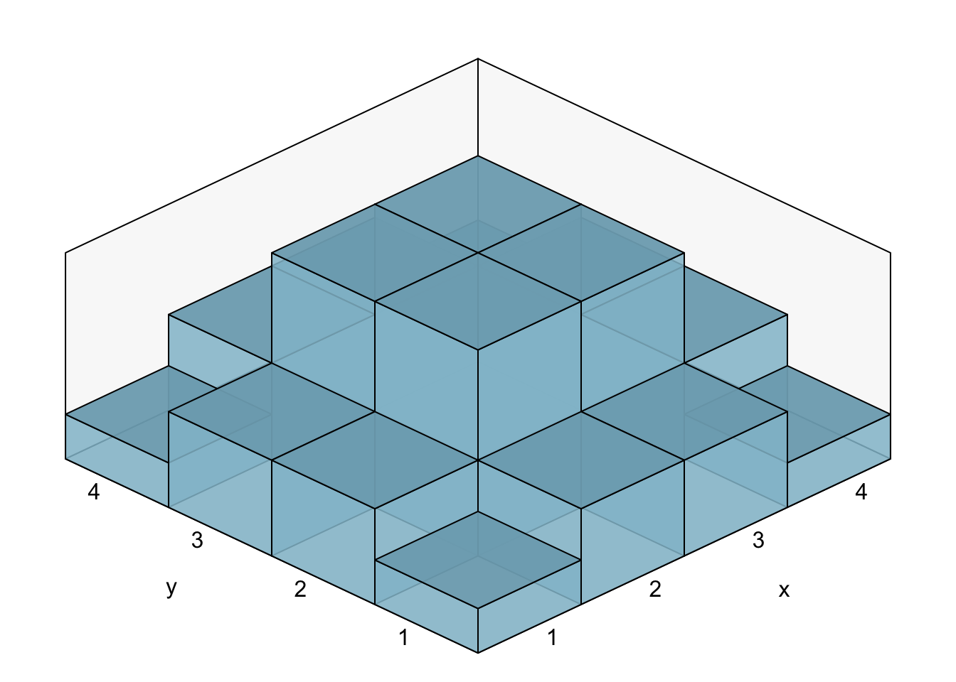
We take this distribution as our null-hypothesis. We generate some data and perform the Chi-square-test:

set.seed(12345)
x <- rnorm(1000)
y <- rnorm(1000)
x_discrete <- cut(x,breaks=c(-10,-1:1, 10))
y_discrete <- cut(y,breaks=c(-10,-1:1, 10))
data <- table(x_discrete, y_discrete)
data

##           y_discrete
## x_discrete (-10,-1] (-1,0] (0,1] (1,10]
##   (-10,-1]       32     44    52     21
##   (-1,0]         55    110   111     53
##   (0,1]          53    138   115     68
##   (1,10]         21     55    48     24

c(data)

##  [1]  32  55  53  21  44 110 138  55  52 111 115  48  21  53  68  24

chisq.test(c(data), p= prob)

## 
##  Chi-squared test for given probabilities
## 
## data:  c(data)
## X-squared = 14.201, df = 15, p-value = 0.5103

qchisq(0.95, df=15)

## [1] 24.99579

As , we (correctly) do not reject the null-hypothesis.

2.3 Case 4a: Bivariate Discrete Distributions With Unknown Parameters

Estimate parameters
apply Chi-squared test with

Instead of describing an example of this case, we will go deeper into the very important test for independence of two discrete random variables. This test turns out to belong to this case 4a (which in itself is almost equal to case 2a).

Testing for Independence in A Contingency Table

An important application of case 4a is testing if two discrete random variables are independent. Two discrete random variables (taking the values ) and (taking the values ) are called independent if

If all the marginal probabilities and were known, we could formulate the null-hypothesis: under the null-hypothesis we would have a Multinomial distribution with known probabilities for .

These marginal probabilities can, however, easily be estimated using the row-totals and column-totals of our observed frequency table:

As , we need only estimate for . As as well, we need only estimate for . Therefore, in total, we need to estimate parameters.

We now have estimates of the probabilities of our bivariate discrete Multinomial distribution if the null-hypothesis is true. From these, we can obtain the expected frequencies:

We are now ready to compute .

Note that the test for independence is simply a special case of case 2a. The degrees of freedom of the Chi-squared test equal , which can be written as :

Under the null-hypothesis, we therefore have

We now have the following method to test for independence of two discrete random variables:

Chi-squared Test: Test for Independence

step 1: and are independent. The random variables and are both discrete ( has groups and has groups).
step 2: Calculate , the expected frequencies if is true, for and . For each , we need .
step 3: Calculate and reject if .

As an example, let’s test if smoking habit is independent of exercising, using the chisq.test command:

library(MASS)       # load the MASS package
head(survey[, c("Exer", "Smoke")]) # first 6 observations of raw data

##   Exer Smoke
## 1 Some Never
## 2 None Regul
## 3 None Occas
## 4 None Never
## 5 Some Never
## 6 Some Never

freq <- table(survey$Smoke, survey$Exer) 
freq         # the contingency table (or: frequency table)

##        
##         Freq None Some
##   Heavy    7    1    3
##   Never   87   18   84
##   Occas   12    3    4
##   Regul    9    1    7

res <- chisq.test(freq)

## Warning in chisq.test(freq): Chi-squared approximation may be incorrect

res

## 
##  Pearson's Chi-squared test
## 
## data:  freq
## X-squared = 5.4885, df = 6, p-value = 0.4828

res$expected

##        
##              Freq      None      Some
##   Heavy  5.360169  1.072034  4.567797
##   Never 92.097458 18.419492 78.483051
##   Occas  9.258475  1.851695  7.889831
##   Regul  8.283898  1.656780  7.059322

The warning message in the output occurs because not all expected frequencies are larger or equal than . We combine the None and Some columns to deal with this:

freq_new = cbind(freq[,"Freq"], freq[,"None"] + freq[,"Some"]) 
freq_new

##       [,1] [,2]
## Heavy    7    4
## Never   87  102
## Occas   12    7
## Regul    9    8

res2 <- chisq.test(freq_new)
res2

## 
##  Pearson's Chi-squared test
## 
## data:  freq_new
## X-squared = 3.2328, df = 3, p-value = 0.3571

res2$expected

##            [,1]      [,2]
## Heavy  5.360169  5.639831
## Never 92.097458 96.902542
## Occas  9.258475  9.741525
## Regul  8.283898  8.716102

As all , we do not get a warning message this time. As the p-value is larger than , we do not reject the null-hypothesis that Smoke and Exer are independent. Note that, as an example, can be calculated as follows:

colSums(freq_new)

## [1] 115 121

rowSums(freq_new)

## Heavy Never Occas Regul 
##    11   189    19    17

2.4 Case 4b: Bivariate Continuous Distributions With Unknown Parameters

Estimate parameters
Discretise
apply Chi-squared test with

Suppose that, in the example of case 3b, we would not have known the values of the two means, the two variances and the covariance. We can still use the Chi-squared test, using the estimated parameters. As in this case, the only change would be the critical value: instead of , we would now have . The parameters are easily estimated

n <- 1000
raw_data <- cbind(x,y)
colMeans(raw_data)

##           x           y 
##  0.04619816 -0.03039248

#maximum likelihood estimator is UNadjusted sample variance/covariance:
((n-1)/n)*var(raw_data)

##            x          y
## x 0.99649932 0.03901121
## y 0.03901121 1.01575949

We would proceed to test the null-hypothesis that has a bivariate Normal distribution with , , , and . As this bivariate Normal distribution is almost equal to the bivariate standard-normal, we do not expect the test to give a different result. In particular, we expect that the value of will again be somewhere between and (it was equal to in the example of case 3b). The critical value can be quite different with :

qchisq(0.95, df=15)

## [1] 24.99579

qchisq(0.95, df=10)

## [1] 18.30704

The null-hypothesis would probably again not be rejected.

Last updated on Jan 1, 0001

Edit this page