1. Introduction to R
1 Installing R and RStudio
- Download and install Base R from r-project or CRAN
- Download and install RStudio Desktop from RStudio
- Start RStudio
If you want to learn more about how to work with RStudio, this is a good start. If you prefer video, you can go here and here. If you are interested in learning more advanced R, I recommend this book.
Installing packages:
For reproducible research, I recommend installing the packages:
- Packages - install - knitr
- Packages - install - tinytex (see documentation. After installing tinytex, you have to run tinytex::install_tinytex() in RStudio).
- Packages - install - rmarkdown
- In RStudio - Preferences (Windows: Tools - Global Options) - Sweave: Weave Rnw-files using: knitr
For the contents of this section, I recommend installing:
- Packages - install - tidyverse (this includes the packages dplyr and ggplot2)
- Packages - install - ggfortify
- Packages - install - manipulate
2 Calculating Probabilities
R has commands that allow you to calculate the value of the pdf, cdf and quantile functions easily for a wide range of distributions (see help for “distributions”). For a distribution named xxx, these commands are named in the form dxxx, pxxx, qxxx, respectively. a random sample from the distribution named xxx can be obtained using rxxx. For example, rnorm(10) draws a random sample of size \(10\) from the standard-normal distribution. For other distributions:
- use xxx=binom for the Binomial distribution.
- use xxx=pois for the Poisson distribution.
- use xxx=norm for the Normal distribution
- use xxx=exp for the Exponential distribution.
- use xxx=unif for the continuous Uniform distribution.
Simulate Random samples
rnorm(10)## [1] 1.0476535 -0.6200811 1.5320591 -0.6000947 0.8383949 -0.7531874
## [7] -0.2089032 0.4867846 -1.3545987 -2.0860992rnorm(10, mean=5, sd=3)## [1] 8.952430 8.813026 4.407189 5.313106 6.080555 6.719318 5.625569 2.747132
## [9] 5.308532 6.496762value of the pdf
dexp(1, rate=1)## [1] 0.3678794value of the cdf
ppois(5, lambda=1)## [1] 0.9994058quantiles
qnorm(0.95, mean=0, sd=1)## [1] 1.6448543 Creating A Graph: R Graphics
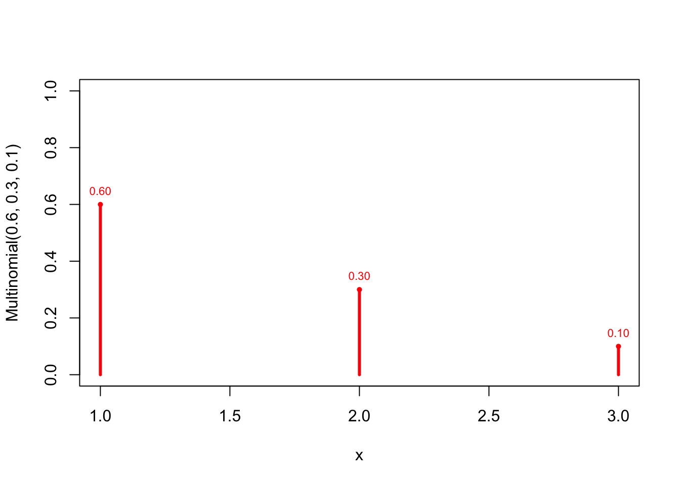
You can use the plot command in R to create graphs. If you have data on two variables x and y, plot(x,y) would create a scatter-plot. Adding the option type=“h” plots vertical lines to the points. The option lwd can be used to change the line-width. Other commands (like points and text) can be used to improve the graph.
x <- 1:3
prob <- c(0.6,0.3,0.1)
plot(x=x, prob, type ="h", lwd=3, col="red", xlab="x",
     ylab="Multinomial(0.6, 0.3, 0.1)", ylim=c(0,1))
points(x, prob, pch=16, cex=0.7, col="red")
text(x, prob, pos=3, cex=0.7, col="red",
     labels = format(round(prob,2), nsmall=2)
     )
4 Creating A Nicer Graph: ggplot2
The R-package ggplot2 has become very popular in R. Like plot, the ggplot command creates graphs. The philosophy behind the ggplot package is quite different from plot, however. It uses the so-called “Grammar of graphics” as its organising principle. You can see an example of its use below.
library(dplyr)
library(ggplot2)

x <- 0:15
lambda = 1
y <- round(dpois(x,lambda),2)
data <- tibble(x,y)
gg <- ggplot(data, aes(x=x, y=y)) +
      geom_point(color="red") +
      geom_text(label = ifelse(y>0, y, ""), size=3, vjust=-0.4) +
      geom_linerange(
        aes(x = x, ymin = 0, ymax = y),
        color = "red", size = 1.0) +
      theme_bw()
gg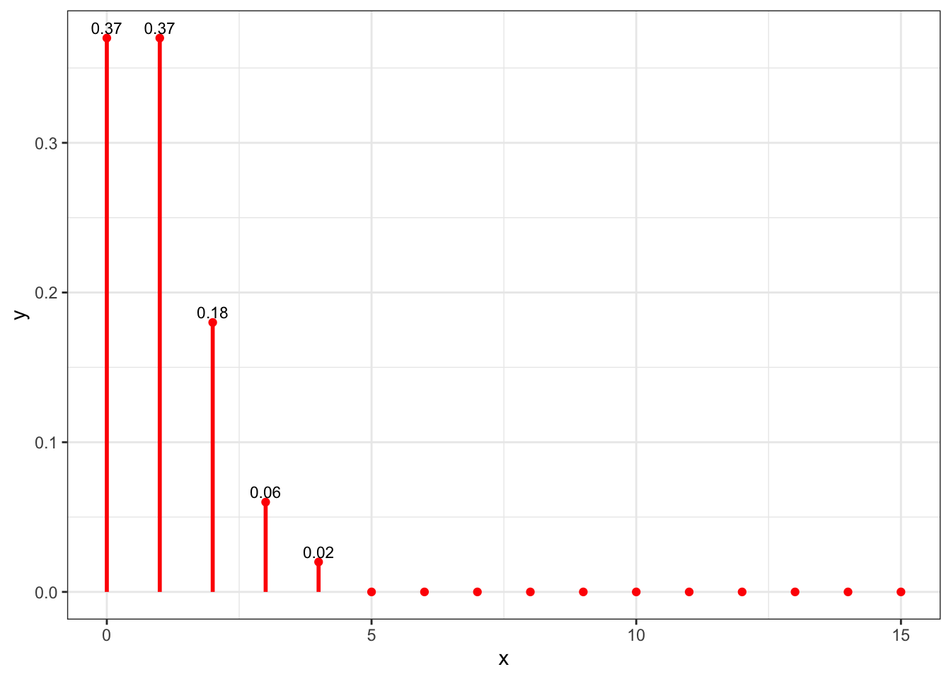
5 Manipulate Graphs Using A Function
R is a programming language. So far, we have used some built-in R commands to calculate probabilities and create graphs. We can, however, also make our own commands. Commands are actually functions: they use some inputs to calculate and return some other outputs. A simple example of a function is:
Creating a Function
add <- function(a,b){
  sum <- a + b
  return(sum)
}
add(5,7)
## [1] 12The function that we have called add takes two arguments, called \(a\) and \(b\). It uses those arguments to calculate the sum, \(a+b\), which is then returned as output. We now give an example of a function that does something more interesting.
Using a Function to Manipulate a Graph
We want to create and show several graphs of the Poisson distribution with different values of the parameter \(\lambda\). Instead of the command lambda <- 1, we create a function of lambda (that we will call graph) and use the manipulate function from the manipulate package to obtain what we want:
library(dplyr)
library(ggplot2)
library(manipulate)

graph <- function(lambda){
  x <- 0:15
  y <- round(dpois(x,lambda),2)
  data <- tibble(x,y)
  gg <- ggplot(data, aes(x=x, y=y)) +
    geom_point(color="red") +
    geom_text(label = ifelse(y>0, y, ""), size=3, vjust=-0.4) +
    geom_linerange(
      aes(x = x, ymin = 0, ymax = y),
      color = "red", size = 1.0) +
    theme_bw()
  gg
}
manipulate(graph(lambda), lambda=slider(1,5,step=0.5))
To manipulate the value of \(\lambda\), click the cogwheel on the left-upper corner of the graph and use the slider. This will only work when you execute the code in RStudio. It is not possible to show you the result in this webpage.
6 More Manipulation Using if-else-statements
An if-statement (or if-else-statement) allows you to choose what the function will do depending on the value of some variable. You essentially create two branches of the program. Which branch will be executed depends on the value of the variable. An easy example of using an if-statement is:
add_mult <- function(type, a, b){
  if (type == "add"){
    return(a + b)
  }
  else{ #type is "multiply"
    return(a * b)
  }
}
add_mult("add", 2, 5)
## [1] 7add_mult("multiply", 2, 5)## [1] 10We can improve our graph function by allowing the user to choose between showing the pdf or the cdf:
library(dplyr)
library(ggplot2)
library(manipulate)

graph <- function(type, lambda){
  x <- 0:15

  if (type == "pdf"){
    y <- round(dpois(x,lambda),2)
  }
  else {
    y <- round(ppois(x,lambda),2)
  }

  data <- tibble(x,y)
  gg <- ggplot(data, aes(x=x, y=y)) +
    geom_point(color="red") +
    geom_text(label = ifelse(y>0, y, ""), size=3, vjust=-0.4) +
    geom_linerange(
      aes(x = x, ymin = 0, ymax = y),
      color = "red", size = 1.0) +
    theme_bw()
  gg
}
manipulate(graph(type, lambda), type=picker("pdf","cdf"), lambda=slider(1,5,step=0.5))
Finally, we create the files discrete.R and continuous.R, so that you can graph any distribution you want. Running the file discrete.R allows you to manipulate discrete distributions with one or two parameters. Running continuous.R does the same for continuous distributions.
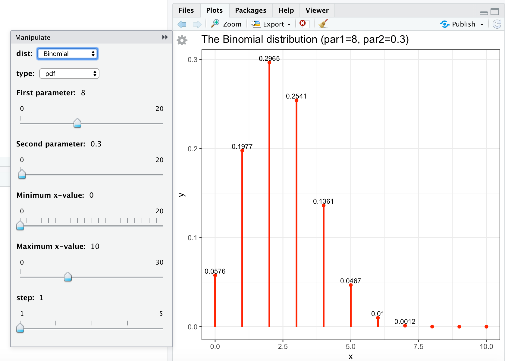
Manipulate Graphs of Discrete Distributions
#save this code (copy paste into file-new file-R script) as discrete.R

library(dplyr)
library(ggplot2)
library(manipulate)

discrete <- function(xmin=0, xmax=20, step=1, dist, type, par1, par2){

  x <- seq(xmin, xmax, step)

  #Poisson distribution
  if (dist == "Poisson"){
    if (type == "pdf"){
      y <- round( dpois(x, par1), 4)
    }
    else {
      y <- round( ppois(x, par1), 4)
    }
  }

  #Binomial distribution
  if (dist == "Binomial"){
    if (type == "pdf"){
      y <- round(dbinom(x, par1, par2), 4)
    }
    if (type == "cdf"){
      y <- round(pbinom(x, par1, par2), 4)
    }
  }

  data <- tibble(x,y)
  gg <- ggplot(data, aes(x=x, y=y)) +
    geom_point(color="red") +
    geom_text(label = ifelse(y>=0.001, y, ""), size=3, vjust=-0.4) +
    geom_linerange(
      aes(x = x, ymin = 0, ymax = y),
      color = "red", size = 1.0) +
    ggtitle(paste("The ", dist, " distribution (par1=", par1, ", par2=", par2,")", sep="")) +
    theme_bw()
  gg
}


# run manipulate once, otherwise the cogwheel doesn't appear
# (bug in manipulate)

manipulate(
  plot(1:x), x = slider(1, 100)
)

manipulate( discrete(xmin, xmax, step, dist, type, par1, par2),
            dist = picker("Poisson", "Binomial"),
            type = picker("pdf","cdf"),
            ###########################################################################################
            ### Change (min,max,step) in (par1, par2) below and source again
            ### to obtain the sliders you want:
            ###########################################################################################
            par1 = slider(min=0, max=20, step=0.1,  label="First parameter", initial=2, ticks=TRUE),
            par2 = slider(min=0, max=1,  step=0.05, label="Second parameter", initial=0.5, ticks=TRUE),
            ###########################################################################################
            xmin = slider(min=0, max=20, step=1, label="Minimum x-value", initial=0, ticks=TRUE),
            xmax = slider(min=0, max=30, step=1, label="Maximum x-value", initial=5, ticks=TRUE),
            step = slider(1, 5, step=1)
            )
You can save this code in discrete.R. The result of running (source) this file will be shown in the Viewer:
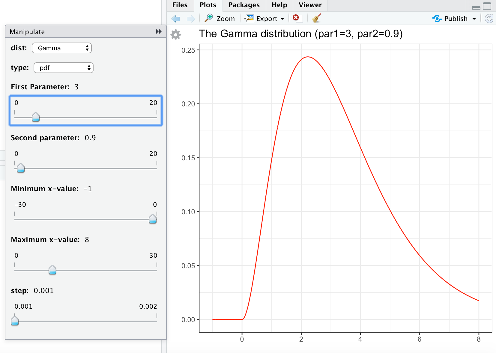
Manipulate Graphs of Continuous Distributions
To graph continuous distributions you can use the code below.
# save this code (copy paste into file-new file-R script) as continuous.R

library(dplyr)
library(ggplot2)
library(manipulate)
library(ggfortify)

continuous <- function(xmin, xmax, step, dist, type, par1, par2){

  x <- seq(xmin, xmax, step)

  #Normal
  if (dist == "Normal"){
    if (type == "pdf"){
      gg <- ggdistribution(dnorm, x, mean = par1, sd = par2, colour = 'red')
    }
    if (type == "cdf"){
      gg <- ggdistribution(pnorm, x, mean = par1, sd = par2, colour = 'blue')
    }
  }

  #t
  if (dist == "t"){
    if (type == "pdf"){
      gg <- ggdistribution(dt, x, df = par1, colour = 'red')
    }
    if (type == "cdf"){
      gg <- ggdistribution(pt, x, df = par1, colour = 'blue')
    }
  }

  #Exponential
  if (dist == "Exponential"){
    if (type == "pdf"){
      gg <- ggdistribution(dexp, x, rate = par1, colour = 'red')
    }
    if (type == "cdf"){
      gg <- ggdistribution(pexp, x, rate = par1, colour = 'blue')
    }
  }

  #Gamma
  if (dist == "Gamma"){
    if (type == "pdf"){
      gg <- ggdistribution(dgamma, x, shape = par1, rate = par2, colour = 'red')
    }
    if (type == "cdf"){
      gg <- ggdistribution(pgamma, x, shape = par1, rate = par2, colour = 'blue')
    }
  }

  #Chi-squared
  if (dist == "Chi-squared"){
    if (type == "pdf"){
      gg <- ggdistribution(dchisq, x, df = par1, colour = 'red')
    }
    if (type == "cdf"){
      gg <- ggdistribution(pchisq, x, df = par1, colour = 'blue')
    }
  }

  #F
  if (dist == "F"){
    if (type == "pdf"){
      gg <- ggdistribution(df, x, df1 = par1, df2 = par2, colour = 'red')
    }
    if (type == "cdf"){
      gg <- ggdistribution(pf, x, df1 = par1, df2 = par2, colour = 'blue')
    }
  }
  gg <- gg +
        ggtitle(paste("The ", dist, " distribution (par1=", par1, ", par2=", par2,")", sep="")) +
        theme_bw()
  return(gg)
}

# run manipulate once, otherwise the cogwheel doesn't appear
# (bug in manipulate)

manipulate(
    plot(1:x), x = slider(1, 100)
)

manipulate( continuous(xmin, xmax, step, dist, type, par1, par2),
            dist = picker("Normal", "t","Exponential", "Gamma", "Chi-squared", "F"),
            type = picker("pdf","cdf"),
            #########################################################################################
            ### Change (min,max,step) in (par1, par2) below and source again
            ### to obtain the sliders you want:
            #########################################################################################
            par1 = slider(min=0, max=20, step=0.1, initial=1, label="First Parameter", ticks = TRUE),
            par2 = slider(min=0, max=20, step=0.1, initial=1, label="Second parameter", ticks=TRUE),
            #########################################################################################
            xmin = slider(min=-30, max=0, step=1, initial=-5, label="Minimum x-value", ticks=TRUE),
            xmax = slider(min=0, max=30, step=1, initial=5, label="Maximum x-value", ticks=TRUE),
            step = slider(0.001, 0.002, step=0.001)
)
You can save these commands in continuous.R. Sourcing this file will give something like