6. Hypothesis Testing

1 The Significance Level and The Power-function of a Statistical Test
2 The Relationship Between Tests and Confidence Intervals
3 Statistical Hypothesis Testing
4 Testing $H_{0} : μ = μ_{0}$ or $H_{0} : p = p_{0}$ .
5 Testing $H_{0} : μ_{1} - μ_{2} = 0$ (or $p_{1} - p_{2} = 0$ )
- 5.1 Example 5: $X_{1} \sim N (μ_{1}, σ_{1}^{2})$ and $X_{2} \sim N (μ_{2}, σ_{2}^{2})$
- 5.2 Example 6: $X_{1} \sim B e r n o u l l i (p_{1})$ and $X_{2} \sim B e r n o u l l i (p_{2})$
6 Testing $H_{0} : σ^{2} = σ_{0}^{2}$
- 6.1 Example 7: $X \sim N (μ, σ^{2})$ :
- 6.2 Aproximation using CLT
7 Testing $H_{0} : \frac{σ_{1}^{2}}{σ_{2}^{2}} = c_{0}$
- 7.1 Example 8: $X_{1} \sim N (μ_{1}, σ_{1}^{2})$ and $X_{2} \sim N (μ_{2}, σ_{2}^{2})$
- 7.2 Aproximation using CLT

This chapter is strongly related to the chapter about confidence intervals. In the confidence interval chapter, we learned how to combine information about our estimator and its RSD to construct a (possibly approximate) $95 %$ (or $99 %$ ) confidence interval for some unknown parameter $θ$ , as in:

$P (2.1 < θ < 3.4) = 0.95.$

In this chapter, we will answer a slightly different question:

Suppose that somebody claims to know that $θ = 5$ (this is called the null-hypothesis).
How can we use our random sample of data (and our assumptions about the population distribution) to detect if this claim is false?
Again, we need to include a quantification of uncertainty due to sampling.

We will see that the end-result of step 2 of the construction of a statistical test is a so-called decision rule. The decision rule of a particular test for a particular problem could for instance be:

Reject the null hypothesis that $θ$ is equal to $5$ if $\bar{X}$ is larger that $7.1$ .

We can then calculate the sample average using our sample of data, and make the decision (this is step 3).

The null-hypothesis $H_{0}$ (pronounce “H nought”) is the statement that we want to test. Suppose that a guy called Pierre claims to know that $θ = 5$ . We then have $H_{0} : θ = 5$ . Testing this null-hypothesis means that we will confront this statement with the information in the data. If it is highly unlikely that we would observe the information in the data that we have observed, under the conditions that are implied by the null hypothesis being true, we reject the null-hypothesis (in other words, “I don’t believe you Pierre”), in favour of the alternative hypothesis, $H_{1} : θ \neq 5$ . If no such statement can be made, we do not reject the null-hypothesis.

A judge in a court of law tests null-hypotheses all the time: in any respectable democracy, the null hypothesis entertained by the judicial system is “suspect is not guilty”. If there is sufficient evidence to the contrary, the judge rejects this null-hypothesis, and the suspect is sent to jail, say. If the judge does not reject the null-hypothesis, it does not mean that the judicial system claims that the suspect is innocent. All it says is that there was not enough evidence against the validity of the null hypothesis. In statistics, as in law, we never accept the null-hypothesis. We either reject $H_{0}$ or we do not reject $H_{0}$ .

1 The Significance Level and The Power-function of a Statistical Test

We will discuss a method to construct statistical tests shortly. For now, suppose that we have constructed a test for $H_{0} : θ = 5$ , and have obtained the following decision rule:

Reject the null hypothesis that $θ$ is equal to $5$ if $\bar{X}$ is larger that $7.1$ .

We cannot be $100 %$ sure that our decision is correct. We can make two types of errors:

We can reject the null-hypothesis when it is, in fact, true (i.e. in reality $θ = 5$ ). This error is called a type-I error. The probability that we make this error is called the level or significance level of the test, and is denoted by $α$ . We want this probabilty to be small. We often take $α = 5 %$ or $α = 1 %$ .
We can fail to reject the null-hypothesis when it is, in fact, false (i.e. in reality $θ \neq 5$ ). This error is called a type-II error. The probability that we make this error is denoted by $β (θ)$ . Note that this is a function of $θ$ : the probability of making a type-II error when the true $θ$ is equal to $5.1$ is different from the probability of making a type-II error when the true $θ$ is equal to $10$ , for instance. The power-function of the test evaluated at $θ$ is defined as $1 - β (θ)$ : it is the probability of (correctly) rejecting the null-hypothesis when it is, in fact, false. We want the power to be high (close to one) for each value $θ \neq 5$ . See Example 1 for an example of a power-function.

2 The Relationship Between Tests and Confidence Intervals

There is a one-to-one relationship between hypothesis testing and confidence intervals; suppose that we have obtained the following $95 %$ confidence interval for $θ$ :

$P (2.1 < θ < 3.4) = 0.95.$

The link with hypothesis testing is as follows:

Suppose that we test $H_{0} : θ = θ_{0}$ , where $θ_{0}$ is some known value. All hypothesis tests that use a value of $θ_{0}$ that is contained within the $95 %$ confidence interval, will not lead to a rejection of $H_{0} : θ = θ_{0}$ at the $α = 5 %$ level.

For instance, from the confidence interval above, we can conclude that $H_{0} : θ = 3.3$ would not be rejected. The null hypothesis $H_{0} : θ = 3.5$ , however, would be rejected. More about this in Example 1.

3 Statistical Hypothesis Testing

We will now discuss the method that can be used to obtain a statistical test that tests the null-hypothesis that $θ = θ_{0}$ , for some pre-specified value of $θ_{0}$ .

The Method: Testing $H_{0} : θ = θ_{0}$ versus $H_{1} : θ \neq θ_{0}$ .

Step 1: Find Pivotal Statistic (or: Test statistic) $T (d a t a | θ_{0})$ .
Step 2: Obtain the quantiles (called critical values now) from $R S D (T)$ under $H_{0}$ . We can now formulate the decision rule.
Step 3: Calculate $T_{o b s}$ and compare with critical values (or use the p-value).

The hardest part is step 1. A pivotal statistic (T) is a function of the data (our random sample) alone, given that we know the value of $θ_{0}$ , the value of the parameter that we want to test. This value $θ_{0}$ is called the hypothesised value of $θ$ . It was $5$ in the example above. It turns out that the pivotal statistic is often equal to the pivotal quantity that we needed to obtain confidence intervals. It is a statistic in the current context, because the value of $θ$ is known (it is $θ_{0}$ ), whereas in confidence intervals it was not known. That is why $P Q (d a t a, θ)$ was called a pivotal quantity, not a pivotal statistic.

The pivotal statistic (or: test statistic) must satisfy the following two conditions:

The distribution of T should be completely known if the null-hypothesis is true (for instance, $N (0, 1)$ or $F_{2, 13}$ ).
T itself should not depend on any parameters that are unknown if the null hypothesis is true (i.e. given that the value of $θ_{0}$ is a known constant). It is only allowed to depend on the data (which is the definition of a statistic).

Condition 1 allows us to perform step 2 of the method.
Condition 2 allows us to perform step 3 of the method.

The easiest way to clarify the method is to apply it to some examples.

4 Testing $H_{0} : μ = μ_{0}$ or $H_{0} : p = p_{0}$ .

For the case that we want to test a null-hypothesis about the mean of a population distribution, we will discuss examples where the population distribution is Bernoulli, Poisson, Normal or Exponential.

4.1 Example 1: $X \sim N (μ, σ^{2})$

We are considering the situation where we are willing to assume that the population distribution is a member of the family of Normal distributions. We are interested in testing the null-hypothesis $H_{0} : μ = μ_{0}$ .

Step 1: Find a Test Statistic (or: Pivotal Statistic) $T (d a t a | μ_{0}) :$

The method requires us to find a pivotal statistic T. As this is a question about the mean of the population distribution, it makes sense to consider the sample average (this is the Method of Moments estimator of $μ$ , as well as the Maximum Likelihood estimator of $μ$ ). We know that linear combinations of Normals are Normal, so that we know the RSD of $\bar{X}$ :

$\bar{X} \sim N (μ, \frac{σ^{2}}{n}) .$ If the null-hypothesis is true, we obtain:

$\bar{X} \underset{H_{0}}{\sim} N (μ_{0}, \frac{σ^{2}}{n}) .$

The quantity $\bar{X}$ is not a pivotal statistic, as the RSD of $\bar{X}$ is not completely known: it depends on the unknown parameter $σ^{2}$ , even given a known value of $μ_{0}$ .

Let’s try standardising with the population-variance:

$\frac{\bar{X} - μ_{0}}{\sqrt{\frac{σ^{2}}{n}}} \underset{H_{0}}{\sim} N (0, 1) .$

The quantity on the left-hand side satisfies the first condition of a pivotal statistic: the standard normal distribution is completely known (i.e. has no unknown parameters). The quantity itself does not satisfy the second condition: although it is allowed to depend on the known $μ_{0}$ , it also depends on the unknown parameter $σ^{2}$ , and is hence not a statistic.

We can solve this problem by standardising with the estimated variance $S^{' 2}$ (instead of $σ^{2}$ ):

$T = \frac{\bar{X} - μ_{0}}{\sqrt{\frac{S^{' 2}}{n}}} \underset{H_{0}}{\sim} t_{n - 1} .$

We have obtained a pivotal statistic $T$ : $T$ itself depends on the sample alone (given that $μ_{0}$ is a known constant if $H_{0}$ is known to be true) and is hence a statistic. Moreover, if $H_{0}$ is true, the RSD of T is completely known. We can progress to step two.

Step 2: Obtain the critical values from $R S D (T)$ under $H_{0}$ .

We need to find the values $a$ and $b$ such that $P (a < T < b) = 0.95$ under $H_{0}$ (i.e. assuming that the null-hypothesis is true). In other words, we need to find the following:

$a = q_{0.025}^{t_{n - 1}}$ : the $2.5 %$ quantile of the $t$ distribution with $n - 1$ degrees of freedom.
$b = q_{0.975}^{t_{n - 1}}$ : the $97.5 %$ quantile of the $t$ distribution with $n - 1$ degrees of freedom.

These are easily found using the statistical tables or by using R. If, for example, we have a sample of size $n = 50$ :

qt(0.025, df=49)

## [1] -2.009575

qt(0.975, df=49)

## [1] 2.009575

As the $t$ distribution is symmetric, it would have sufficed to calculate only one of the two quantiles.

We have the following decision rule:

Reject the null hypothesis if the observed test-statistic is larger than 2.009575 or smaller than -2.009575.

One-sided Tests: We have been using the two-sided alternative hypothesis $θ \neq θ_{0}$ in this example. Sometimes we prefer the right-sided (or left-sided) alternative hypothesis $θ > θ_{0}$ ( $θ < θ_{0}$ ).

In that case, there would be evidence against the null-hypothesis if ${\bar{X}}_{o b s}$ is a sufficient amount larger than $θ_{0}$ (a sufficient amount smaller than $θ_{0}$ ), which implies that $T_{o b s}$ is sufficiently positive (negative).

What constitutes sufficiently positive (negative)? With

α = 5 %

, a value of

T_{o b s}

larger than

q_{0.95}^{t_{n - 1}}

(smaller than

q_{0.05}^{t_{n - 1}}

) would be considered sufficiently unlikely to have ocurred under the null hypothesis.

In our example, the alternative hypothesis $θ > 5$ would therefore have led to the following decison-rule:

Reject the null hypothesis if the observed test-statistic is larger than 1.676551.

We test $θ = θ_{0}$ against $θ > θ_{0}$ if we are $100 %$ sure that $θ$ is not smaller than $θ_{0}$ . Likewise, we test $θ = θ_{0}$ against $θ < θ_{0}$ if we are $100 %$ sure that $θ$ is not larger than $θ_{0}$ .

The link between Hypothesis Testing and Confidence Intervals:

To understand this link, let’s focus on the following true statement (we consider the two-sided test):

$If H_{0} is true, P (q_{0.025}^{t_{n - 1}} < \frac{\bar{X} - μ_{0}}{\sqrt{\frac{S^{' 2}}{n}}} < q_{0.975}^{t_{n - 1}}) = 0.95.$

Note that, if we replace $μ_{0}$ by $μ$ , this probability is true for any value of $μ$ that is contained in the confidence interval (by step 3 of the confidence interval method).
Therefore, any hypothesised value $μ_{0}$ that is contained within the confidence interval will not be rejected by the test.

Step 3: Calculate $T_{o b s}$ and compare with critical values.

Using a sample of size $n = 50$ , we can calculate the values of $\bar{X}$ and $S^{' 2}$ . As the value of $μ_{0}$ is known, the pivotal statistic is truly a statistic: it is a function of the random sample alone. Because we have observed a random sample from the population distribution, we can calculate the value that $T$ takes using our observed sample: $T_{o b s}$ . Suppose that we obtain $T_{o b s} = 3.4$ , using a sample of size $n = 50$ .

The argument of a statistical test is as follows:

In step 2, we have derived that, if $H_{0}$ is true, our observed test statistic $T_{o b s}$ is a draw from the $t_{49}$ distribution.
Observing a value $T_{o b s} = 3.4$ from the $t_{49}$ is highly unlikely: $3.4 > 2.01$ , which is the $97.5 %$ quantile of the $t_{49}$ distribution.
We therefore think that the null-hypothesis is false: we reject $H_{0}$ .

To give an example, suppose that we want to test the null-hypothesis $H_{0} : μ = 5$ against the two-sided alternative hypothesis $H_{1} : μ \neq 5$ .

We draw a random sample of size $50$ from $N (μ = 7, σ^{2} = 100)$ . This means that, in reality, the null-hypothesis is false.

set.seed(12345)
data <- rnorm(50, mean=7, sd=10)
data

##  [1]  12.8552882  14.0946602   5.9069669   2.4650283  13.0588746 -11.1795597
##  [7]  13.3009855   4.2381589   4.1584026  -2.1932200   5.8375219  25.1731204
## [13]  10.7062786  12.2021646  -0.5053199  15.1689984  -1.8635752   3.6842241
## [19]  18.2071265   9.9872370  14.7962192  21.5578508   0.5567157  -8.5313741
## [25]  -8.9770952  25.0509752   2.1835264  13.2037980  13.1212349   5.3768902
## [31]  15.1187318  28.9683355  27.4919034  23.3244564   9.5427119  11.9118828
## [37]   3.7591342  -9.6205024  24.6773385   7.2580105  18.2851083 -16.8035806
## [43]  -3.6026555  16.3714054  15.5445172  21.6072940  -7.1309878  12.6740325
## [49]  12.8318765  -6.0679883

We calculate the sample average and the adjusted sample variance:

xbar <- mean(data)
xbar

## [1] 8.795663

S2 <- var(data)
S2

## [1] 120.2501

We calculate the quantiles (it turns out that we only need $b$ ):

b <- qt(0.975, df=49)
b

## [1] 2.009575

The observed value of the test-statistic $T_{o b s}$ is equal to:

T_obs <- (xbar - 5)/sqrt(S2/50)
T_obs

## [1] 2.447541

As $T_{o b s} = 2.4475 > 2.01$ , we reject $H_{0} : μ = 5$ . The test gives the correct result.

The t.test command can do the calculations for us:

t.test(data, mu=5, alternative="two.sided", conf.level=0.95)

## 
##  One Sample t-test
## 
## data:  data
## t = 2.4475, df = 49, p-value = 0.01801
## alternative hypothesis: true mean is not equal to 5
## 95 percent confidence interval:
##   5.67920 11.91213
## sample estimates:
## mean of x 
##  8.795663

The p-value associated with $T_{o b s}$ :

The p-value for a two-sided test (which is shown in the output) is defined as follows:

$p - v a l u e = P (| T | > T_{o b s}) = P (T < - 2.4475) + P (T > 2.4475) .$

We reject a null-hypothesis if the p-value is smaller than $α$ (0.05 here). The conclusion will be the same as the conclusion obtained from comparing $T_{o b s}$ with critical values (step 3). The p-value above actually tells us something more: we would not have rejected the null-hypothesis for a two-sided alternative with $α = 1 %$ . If you use the p-value, there is no need to find critical values (step 2).

If our alternative hypothesis was $μ > μ_{0}$ , we would have used the p-value for a right-sided test:

$p - v a l u e = P (T > T_{o b s}) = P (T > 2.4475) .$

4.1.1 Aproximation using CLT

We are considering the same example, but now we are not willing to assume that the population distribution is a member of the family of Normal distributions. We are still interested in testing $H_{0} : μ = 5$ against the two-sided alternative $H_{1} : μ \neq 5$ .

The narrative does not have to be changed much:

Step 1: Find a Test-statistic (or: pivotal statistic) $T (d a t a | μ_{0})$ :

The method requires us to find a pivotal statistic. For the sample average, we know that, by central limit theorem, that

$\bar{X} \overset{a p p r o x}{\sim} N (μ, \frac{σ^{2}}{n}) .$

We can obtain a test-statistic by standardising with the estimated variance:

$T = \frac{\bar{X} - μ_{0}}{\sqrt{\frac{S^{' 2}}{n}}} \overset{a p p r o x}{\sim} N (0, 1) if H_{0} is true .$

Step 2: Find the critical values $a$ and $b$ with $Pr (a < T < b) = 0.95$ .

The $97.5 %$ quantile of the standard normal distribution is:

b2 <- qnorm(0.975, mean=0, sd=1)
b2

## [1] 1.959964

We can therefore write down the decision rule:

Reject the null hypothesis if the observed test-statistic is larger than 1.96 or smaller than -1.96,

where $T_{o b s} = \frac{{\bar{X}}_{o b s} - μ}{\sqrt{\frac{S^{' 2}}{n}}}$ .

Step 3: Calculate $T_{o b s}$ and compare with critical values (or use the p-value).

We will use the same dataset, so we obtain the same observed test-statistic: $T_{o b s} = 2.447541$ . Note that the data were generated using $μ = 7$ , so that the null-hypothesis is, in fact, false. As $T_{o b s} > 1.96$ , we reject the null-hypothesis (correctly).

The power at $μ = 7$ :

In reality, we would not know for sure that our conclusion is correct, because we would not know that the true mean is equal to 7. The power at $μ = 7$ tells us how likely it is that we draw the correct conclusion using our test when, in fact, $μ = 7$ .

The top graph in the following figure gives a graphical explanation of Power( $μ = 7$ ):

## Using poppler version 0.73.0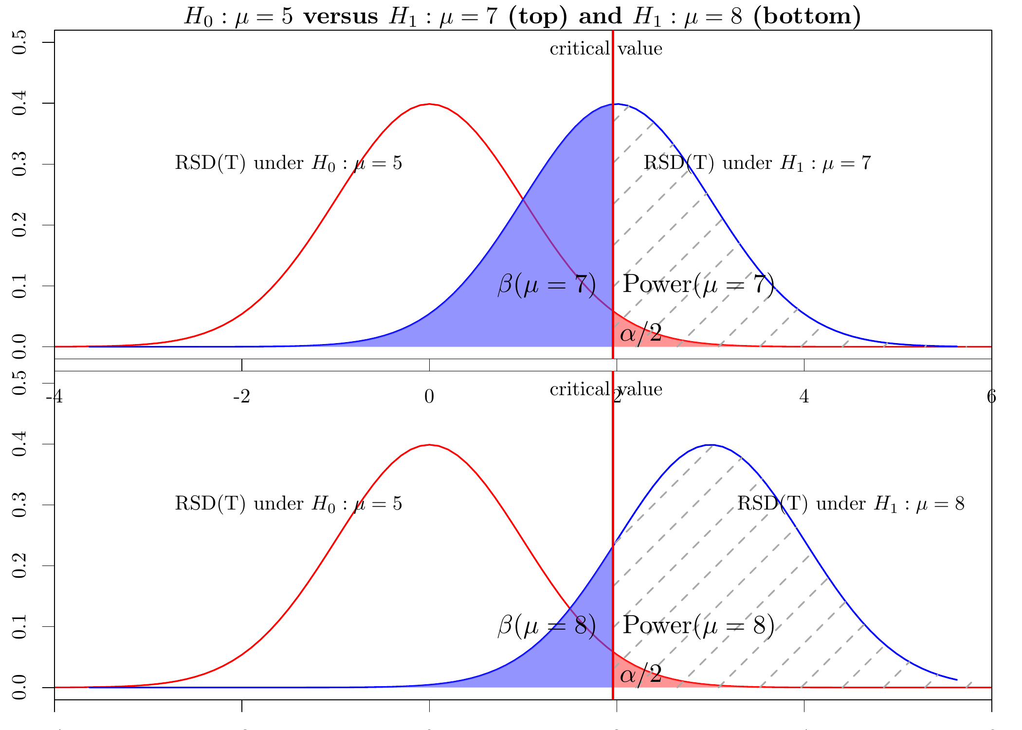

If the null-hypothesis is true, the RSD of T is the standard-normal distribution. If, in reality, $μ = 7$ , the RSD of T is $N (2, 1)$ . Therefore, the Power at $μ = 7$ is the area with dashed diagonal gray lines:

$P o w e r (μ = 7) = P (We reject H_{0} | μ = 7) = P (T < - 1.96 or T > 1.96 | μ = 7) .$

The bottom graph in the figure shows that the power at $μ = 8$ is higher than the power at $μ = 7$ : as the RSD of T is shifted more to the right and the critical value does not change, the area with dashed diagonal gray lines increases.

Plotting the Power-curve

We want to plot the power-curve of our statistical test.

The Power-curve (the power at any $μ \neq μ_{0}$ ):

The power-curve is a plot of the power-function. The power-function of the test is equal to the probability that we reject the null hypothesis, given that it is indeed false. As the null-hypothesis $μ = μ_{0}$ can be false in many ways (it is false whenever the true $μ$ is unequal to $μ_{0}$ , which is 5 in our example), the power of the test is a function of $μ$ :

$P o w e r (μ) = P (We reject H_{0} | μ \neq μ_{0}) .$

We want these probabilities to be as high as possible (or, equivalently, we want the probability of making a type-II error

β (μ)

to be as small as possible) for all values of

μ \neq μ_{0}

In our example, the power-function is equal to

$\begin{aligned} P o w e r (μ) & = P (T < - 1.96 or T > 1.96 | μ \neq μ_{0} is the true value of E [X]) \\ = 1 - P (- 1.96 < \frac{\bar{X} - 5}{\sqrt{120.2501 / 50}} < 1.96 | μ \neq μ_{0} is the true value of E [X]) \\ = 1 - P (- 1.96 < N (μ - 5, 1) < 1.96) \\ = 1 - {Φ (1.96 - (μ - 5)) - Φ (- 1.96 - (μ - 5))} \\ = 1 - Φ (6.96 - μ) + Φ (2.96 - μ) . \end{aligned}$

The two-but-last line uses the symbolic notation $N (μ - 5, 1)$ for a random variable that has the $N (μ - 5, 1)$ distribution. This distribution is obtained from noting that if $μ = 7$ , for instance, the RSD of $\bar{X}$ is $N (7, \frac{σ^{2}}{n})$ , so that $T \overset{a p p r o x}{\sim} N (2, 1)$ . Therefore, for general values of $μ$ , $T \overset{a p p r o x}{\sim} N (μ - 5, 1)$ . To obtain the required probabilities, we substract the mean in the next step to obtain a standard-normal distribution. We now plot the power-function using R:

mu <- seq(from=0, to=10, by=0.1)
mu

##   [1]  0.0  0.1  0.2  0.3  0.4  0.5  0.6  0.7  0.8  0.9  1.0  1.1  1.2  1.3  1.4
##  [16]  1.5  1.6  1.7  1.8  1.9  2.0  2.1  2.2  2.3  2.4  2.5  2.6  2.7  2.8  2.9
##  [31]  3.0  3.1  3.2  3.3  3.4  3.5  3.6  3.7  3.8  3.9  4.0  4.1  4.2  4.3  4.4
##  [46]  4.5  4.6  4.7  4.8  4.9  5.0  5.1  5.2  5.3  5.4  5.5  5.6  5.7  5.8  5.9
##  [61]  6.0  6.1  6.2  6.3  6.4  6.5  6.6  6.7  6.8  6.9  7.0  7.1  7.2  7.3  7.4
##  [76]  7.5  7.6  7.7  7.8  7.9  8.0  8.1  8.2  8.3  8.4  8.5  8.6  8.7  8.8  8.9
##  [91]  9.0  9.1  9.2  9.3  9.4  9.5  9.6  9.7  9.8  9.9 10.0

y <- 1 - pnorm( 6.96 - mu) + pnorm( 2.96 - mu)
y

##   [1] 0.99846180 0.99788179 0.99710993 0.99609297 0.99476639 0.99305315
##   [7] 0.99086253 0.98808937 0.98461367 0.98030073 0.97500211 0.96855724
##  [13] 0.96079610 0.95154278 0.94062007 0.92785499 0.91308508 0.89616539
##  [19] 0.87697572 0.85542791 0.83147274 0.80510607 0.77637368 0.74537467
##  [25] 0.71226284 0.67724599 0.64058294 0.60257833 0.56357538 0.52394672
##  [31] 0.48408404 0.44438669 0.40525008 0.36705437 0.33015398 0.29486860
##  [37] 0.26147601 0.23020706 0.20124304 0.17471547 0.15070815 0.12926136
##  [43] 0.11037777 0.09402971 0.08016731 0.06872703 0.05964005 0.05284013
##  [49] 0.04827045 0.04588912 0.04567306 0.04762015 0.05174936 0.05809910
##  [55] 0.06672357 0.07768766 0.09106026 0.10690664 0.12528008 0.14621336
##  [61] 0.16971050 0.19573926 0.22422494 0.25504581 0.28803058 0.32295817
##  [67] 0.35955989 0.39752390 0.43650205 0.47611856 0.51598016 0.55568737
##  [73] 0.59484605 0.63307886 0.67003594 0.70540430 0.73891544 0.77035107
##  [79] 0.79954646 0.82639161 0.85083028 0.87285699 0.89251238 0.90987737
##  [85] 0.92506633 0.93821984 0.94949743 0.95907050 0.96711588 0.97381016
##  [91] 0.97932484 0.98382262 0.98745454 0.99035813 0.99265637 0.99445738
##  [97] 0.99585470 0.99692804 0.99774432 0.99835894 0.99881711

plot(mu, y, type="l", xlab="mu", ylab="P(reject H0 | mu)", col="blue")

abline(v=7, b=0, col="red")
abline(a=0.05, b=0, lty="dashed", col="gray")
abline(a=0.5159802, b=0, lty="dashed", col="gray")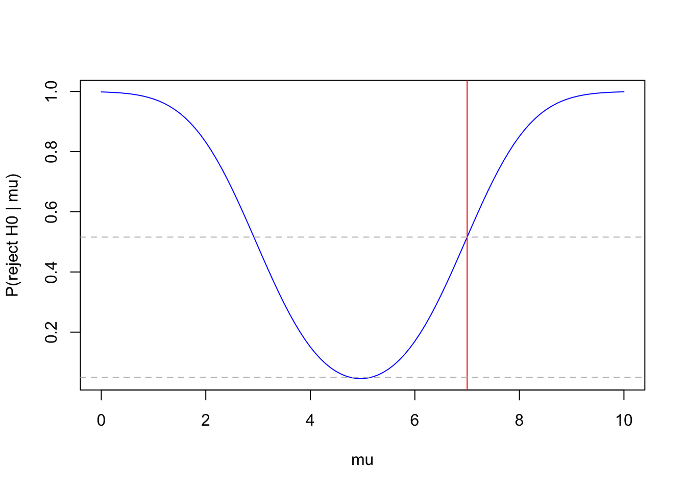

The power-curve shows that we were quite lucky: if $μ = 7$ , the test correctly rejects the null-hypothesis in only about $52 %$ of the repeated samples. Our observed sample was one of those, but need not have been. If, in reality, $μ > 10$ or $μ < 0$ , the test would always give the correct answer.

Note that if in reality $μ = 5$ (i.e. the null hypothesis is true) the test rejects only in $5 %$ of the repeated samples. This is the meaning of $α$ , the probability of a type-I error. Note also that the probability of a type-II error if $μ = 7$ ( $β (7)$ ) is around $48 %$ .

If the alternative hypothesis was $μ > 5$ , the power curve would look different:

$\begin{aligned} P o w e r (μ) & = P (T > 1.645 | μ \neq μ_{0} is the true value of E [X]) \\ = 1 - P (\frac{\bar{X} - 5}{\sqrt{120.2501 / 50}} < 1.645 | μ \neq μ_{0} is the true value of E [X]) \\ = 1 - P (N (μ - 5, 1) < 1.645) \\ = 1 - Φ (1.645 - (μ - 5)) \\ = 1 - Φ (6.645 - μ) . \end{aligned}$

The power-curve of a right-sided test does not increase on the left:

mu <- seq(from=0, to=10, by=0.1)
y <- 1 - pnorm(6.645 - mu)
y2 <- 1 - pnorm( 6.96 - mu) + pnorm( 2.96 - mu)

plot(mu, y, type="l", xlab="mu", ylab="P(reject H0 | mu)")
lines(mu, y2, lty="dashed", col="blue")

abline(v=7, b=0, col="red")
abline(a=0.05, b=0, lty="dashed", col="gray")
abline(a=0.6387052, b=0, lty="dashed", col="gray")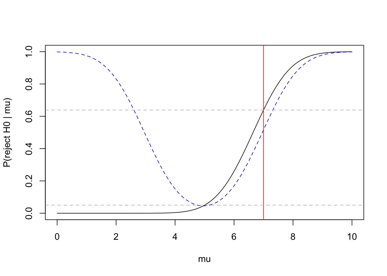

1 - pnorm(6.645 - 7)

## [1] 0.6387052

The power of the right-sided test at $μ = 7$ is about $64 %$ , higher than the $52 %$ for the two-sided test. The power-curve of the two-sided test is plotted in dashed blue for comparison.

4.2 Example 2: $X \sim P o i s s o n (λ)$

We are considering the situation where we are willing to assume that the population distribution is a member of the family of Poissson( $λ$ ) distributions. As the Poisson distribution has $E [X] = λ$ , we are interested in testing $H_{0} : λ = λ_{0}$ versus $H_{1} : λ \neq λ_{0}$ . As an example, we take $n = 100$ and $λ_{0} = 0.2$ .

Step 1: Find a Test-statistic (or: pivotal statistic) $T (d a t a | λ_{0})$ :

The method requires us to find a pivotal statistic $T$ . One requirement is that the T is a statistic (depends only on the data) given that $λ_{0}$ is a known constant (the hypothesised value). It therefore makes sense to consider the sample average (this is the Method of Moments estimator of $λ$ , as well as the Maximum Likelihood estimator of $λ$ ). We do not know the repeated sampling distribution of $\bar{X}$ in this case. All we know is that

$\sum_{i = 1}^{n} X_{i} \sim P o i s s o n (n λ) .$

If the null-hypothesis is true, we have $\sum_{i = 1}^{n} X_{i} \underset{H_{0}}{\sim} P o i s s o n (n λ_{0}) = P o i s s o n (20) .$

This is a pivotal statistic: the RSD of the sum is completely known if we know that $λ_{0} = 0.2$ , and the sum itself is a statistic. We can proceed to step 2.

Step 2: Find the critical values $a$ and $b$ with $Pr (a < T < b) = 0.95$ .

The $2.5 %$ and $97.5 %$ quantiles of the Poisson(20) distribution are (approximately):

a <- qpois(0.025, lambda=20)
a

## [1] 12

b <- qpois(0.975, lambda=20)
b

## [1] 29

ppois(12, 20) #P(T<=12)

## [1] 0.03901199

ppois(11,20)  #P(T<12)

## [1] 0.02138682

1-ppois(29, 20) #P(T>29)

## [1] 0.02181822

1-ppois(28, 20) #P(T>=29)

## [1] 0.03433352

We can therefore write down the decision rule:

Reject the null hypothesis if $\sum_{i = 1}^{n} X_{i}$ is smaller than 12 or larger than 29.

Step 3: Calculate $T_{o b s}$ and compare with critical values (or use the p-value).

We draw a sample of size 100 from the Poisson( $λ = 0.2$ ) distribution, and calculate the sum:

set.seed(1234)
data <- rpois(100, 0.2)
data

##   [1] 0 0 0 0 1 0 0 0 0 0 0 0 0 1 0 1 0 0 0 0 0 0 0 0 0 0 0 1 1 0 0 0 0 0 0 0 0
##  [38] 0 2 0 0 0 0 0 0 0 0 0 0 0 0 0 0 0 0 0 0 0 0 1 1 0 0 0 0 0 0 0 0 0 0 1 0 0
##  [75] 0 0 0 0 0 0 1 0 0 0 0 1 0 0 0 1 0 1 0 0 0 0 0 0 0 0

T_obs <- sum(data)
T_obs

## [1] 14

As $T_{o b s} = 14$ , we do not reject the null-hypothesis that $λ = 0.2$ .

4.2.1 Aproximation using CLT

We are now interested in finding an approximate test for $H_{0} : λ = 0.2$ . There is no good reason to do this, other than checking how good the approximation is.

Step 1: Find a Test-statistic (or: pivotal statistic) $T (d a t a | λ_{0})$ :

As $E [X] = V a r [X] = λ$ for Poisson( $λ$ ) distributions, the central limit theorem states that

$\hat{λ} = \bar{X} \overset{a p p r o x}{\sim} N (λ, \frac{λ}{n}) .$ If the null-hypothesis is true, we have

$\hat{λ} = \bar{X} \overset{a p p r o x}{\sim} N (λ_{0}, \frac{λ_{0}}{n}) = N (0.2, 0.002) .$

We can now standardise:

$\frac{\bar{X} - 0.2}{\sqrt{0.002}} \overset{a p p r o x}{\sim} N (0, 1) .$

This is a pivotal statistic.

Step 2: Find the quantiles $a$ and $b$ such that $Pr (a < T < b) = 0.95$ .

qnorm(0.975)

## [1] 1.959964

The decision rule is:

Reject the null-hypothesis if T<-1.96 ot T>1.96

Note that, as $- 1.96 < T < 1.96$ is equivalent to

$11.23 = 100 (0.2 - \sqrt{0.002} \times 1.96) < \sum_{i = 1}^{n} X_{i} < 100 (0.2 + \sqrt{0.002} \times 1.96) = 28.76,$

we can also write:

Reject the null-hypothesis if $\sum_{i = 1}^{n} X_{i}$ is smaller than 11.23 or larger than 28.77.

This is quite similar to the exact test derived above.

Step 3: Calculate $T_{o b s}$ and compare with critical values (or use the p-value).

Using the same sample, we obtain:

T_obs <- (mean(data) - 0.2)/sqrt(0.002)
T_obs

## [1] -1.341641

As $T_{o b s} = - 1.34$ is not smaller than $- 1.96$ , we do not reject the null-hypothesis that $λ = 0.2$ .

We can also use the p-value:

pnorm(T_obs) + (1-pnorm(-T_obs))

## [1] 0.1797125

As the p-value is not smaller than $0.05$ , we do not reject the null-hypothesis.

4.3 Example 3: $X \sim E x p (λ)$

We are considering the situation where we are willing to assume that the population distribution is a member of the family of Exponential distributions with (unknown) parameter $λ$ . As the exponential distribution has $E [X] = \frac{1}{λ}$ , we are interested in testing $H_{0} : \frac{1}{λ} = \frac{1}{λ_{0}}$ versus the alternative hypothesis $H_{1} : \frac{1}{λ} \neq \frac{1}{λ_{0}}$ . As an example, we will take $λ = 0.2$ and $n = 100$ . Hence, we want to test the null-hypothesis that $E [X] = 5$ .

Step 1: Find a test statistic $T (d a t a | λ_{0})$ :

The parameter $λ$ can be estimated by $\hat{λ} = \frac{1}{\bar{X}}$ , the Method of Moments and Maximum Likelihood estimator. We cannot obtain the exact RSD for this statistic. As we have a random sample from the Exponential distribution, we also know that

$\sum_{i = 1}^{n} X_{i} \sim G a m m a (n, λ) .$

If the null-hypothesis is true, we obtain

$\sum_{i = 1}^{n} X_{i} \underset{H_{0}}{\sim} G a m m a (n, λ_{0}) .$

This is a pivotal statistic. We cannot get the critical values of this statistic using our Statistical Tables. We can transform the Gamma distribution to a chi-squared distribution (for which we have tables) as follows:

$T = 2 λ_{0} \sum_{i = 1}^{n} X_{i} \underset{H_{0}}{\sim} χ_{2 n}^{2} .$

This is also a pivotal statistic.

Step 2: Find the quantiles $a$ and $b$ such that $Pr (a < T < b) = 0.95$ .

The $2.5 %$ and $97.5 %$ quantiles are:

a <- qchisq(0.025, df=200)
a

## [1] 162.728

b <- qchisq(0.975, df=200)
b

## [1] 241.0579

The decision rule is:

Reject the null-hypothesis if $0.4 \sum_{i = 1}^{n} X_{i}$ is smaller than 162.728 or larger than 241.0579.

Reject the null-hypothesis if_{i=1}^n X_i$ is smaller than 406.82 or larger than 602.65.

Step 3: Calculate $T_{o b s}$ and compare with critical values (or use the p-value).

We draw a sample of size 100 from the Exp( $λ = 0.2$ ) distribution, and calculate the sum:

set.seed(12432)
data <- rexp(100, rate=0.2)
data

##   [1]  0.14907795  8.07766447  2.02745666  6.49205265  0.37654896 10.23011103
##   [7]  6.50703386  1.99843257  3.19968787  3.81472730 11.59536625  3.10470183
##  [13]  6.22892454  2.70810540  4.79461150  8.46509304  0.30120264  3.05038690
##  [19]  7.29538310  0.16704212  6.78359305  2.21707233  5.15083448  0.73830057
##  [25]  5.53390365 10.54390572  0.55507295  4.18100134  7.73419513  9.33628288
##  [31]  1.47064050 17.69536803  6.77209163  3.69946593  4.18173227  7.68760043
##  [37]  1.43140818  0.18152633 11.45252555  0.21562584  1.87887548  4.99501155
##  [43]  5.55790541  0.26258148  0.23179928  2.08911416  0.42976580  1.64560789
##  [49]  1.08356090  1.38374444  3.20642702  2.58905530  3.80587957  1.21345423
##  [55]  0.68163493  1.13175232  9.19108407  0.75484126  1.45888929  9.99728440
##  [61]  0.05778570  2.27937926  3.96084369  6.18156264  1.94891606  2.39714234
##  [67]  0.29781575  0.09192151  3.68075910  0.18130849  4.54638749  1.82050722
##  [73]  3.66988372  4.97436924 12.16494984  2.34126599  4.06593290  5.68069283
##  [79]  1.84244461  0.74156984  2.69434477  4.86109398  3.51903898 14.82506115
##  [85]  0.91001743  0.03604018  5.18614162  2.99553917  2.26465601  1.79149822
##  [91]  6.80382571  2.76859507  3.60379507  2.90056841  4.64767496  0.50438227
##  [97] 12.26700920  9.39569936  2.13883634  0.02376590

T_obs <- sum(data)
T_obs

## [1] 398.797

As $T_{o b s} = 398.797$ , we reject the null-hypothesis that $E [X] = 5$ (or that $λ_{0} = 0.2$ ). Note that the null-hypothesis is, in fact, true, as our data was generated using $λ = 0.2$ . We have incorrectly rejected the null hypothesis. As $α = 0.05$ , we know that this type-I error occurs in $5 %$ of the repeated samples. Unfortunately, our observed sample was one of those $5 %$ . In practice, we would not have known this, so we would not have known that we made the wrong decision.

4.3.1 Aproximation using CLT

We will now derive the test using a large sample approximation.

Step 1: Find a pivotal statistic $T (d a t a | λ_{0})$ :

If we have a random sample from the Exponential distribution, which has $E [X] = \frac{1}{λ}$ and $V a r [X] = \frac{1}{λ^{2}}$ , the CLT states that

$\bar{X} \overset{a p p r o x}{\sim} N (\frac{1}{λ}, \frac{1}{n λ^{2}}) .$

If the null-hypothesis is true, we obtain

$\bar{X} \overset{a p p r o x}{\sim} N (\frac{1}{λ_{0}}, \frac{1}{n λ_{0}^{2}}) = N (5, 0.25) .$

We can standardise to obtain a standard-normal distribution (for which we have tables):

$T = \frac{\bar{X} - 5}{\sqrt{0.25}} \underset{H_{0}}{\overset{a p p r o x}{\sim}} N (0, 1) .$

Step 2: Find the quantiles $a$ and $b$ such that $Pr (a < T < b) = 0.95$ .

As before, the $97.5 %$ quantile of $N (0, 1)$ is (more or less) 1.96.

The decision rule is:

Reject the null-hypothesis if T < -1.96 or larger than 1.96.

Note that, as $- 1.96 < T < 1.96$ is equivalent to

$402 = 100 (5 - \sqrt{0.25} \times 1.96) < \sum_{i = 1}^{n} X_{i} < 100 (5 + \sqrt{0.25} \times 1.96) = 598,$

we can also write:

Reject the null-hypothesis if $\sum_{i = 1}^{n} X_{i}$ is smaller than 402 or larger than 598.

This is very similar to the exact test that uses $406.82$ and $602.65$ .

Step 3: Calculate $T_{o b s}$ and compare with critical values (or use the p-value).

Using the same sample we obtain

T_obs <- (mean(data) - 5)/sqrt(0.25)
T_obs

## [1] -2.024059

pnorm(T_obs) + (1-pnorm(-T_obs))

## [1] 0.04296408

As the p-value is smaller than $0.05$ , we reject the null-hypothesis that $E [X] = 5$ . Hence, the approximate test gives the incorrect result, as did the exact test.

4.4 Example 4: $X \sim B e r n o u l l i (p)$

We are considering the situation where we are willing to assume that the population distribution is a member of the family of Bernoulli distributions. We are interested in testing $H_{0} : p = p_{0}$ versus $p \neq p_{0}$ . As an example, we take $n = 100$ and $p = 0.7$ .

Both the Method of Moments estimator and the Maximum Likelihood for $p$ are equal to the sample average.

Step 1: Find a pivotal statistic $T (d a t a | p_{0})$ :

When sampling from the Bernoulli( $p$ ) distribution, we only have the following result:

$\sum_{i = 1}^{n} X_{i} \sim B i n o m i a l (n, p) .$

If the null-hypothesis is true, we obtain

$T = \sum_{i = 1}^{n} X_{i} \sim B i n o m i a l (n = 100, 0.7) .$

As $\sum_{i = 1}^{n} X_{i}$ is a statistic and its distribution is completely known if the null-hypothesis is true, it is a test-statistic.

Step 2: Find the critical values $a$ and $b$ with $Pr (a < T < b) = 0.95$ .

The $2.5 %$ and $97.5 %$ quantiles of the Binomial(n=100, p=0.7) distribution are (approximately):

a <- qbinom(0.025, size=100, prob=0.7)
a

## [1] 61

b <- qbinom(0.975, size=100, prob=0.7)
b

## [1] 79

pbinom(61, size=100, prob=0.7) #P(T<=61)

## [1] 0.033979

pbinom(60, size=100, prob=0.7) #P(T<61)

## [1] 0.02098858

1 - pbinom(79, size=100, prob=0.7) #P(T>79)

## [1] 0.01646285

1 - pbinom(78, size=100, prob=0.7) #P(T>=79)

## [1] 0.02883125

We can therefore write down the decision rule:

Reject the null hypothesis if $\sum_{i = 1}^{n} X_{i}$ is smaller than 61 or larger than 79.

Step 3: Calculate $T_{o b s}$ and compare with critical values (or use the p-value).

We draw a sample of size 100 from the Bernoulli( $p_{0} = 0.7$ ) distribution, and calculate the sum:

set.seed(12345)
data <- rbinom(100, size=1, prob=0.7)
data

##   [1] 0 0 0 0 1 1 1 1 0 0 1 1 0 1 1 1 1 1 1 0 1 1 0 0 1 1 1 1 1 1 0 1 1 1 1 1 0
##  [38] 0 1 1 0 1 0 0 1 1 1 1 1 1 0 0 1 1 0 1 0 1 1 1 0 1 0 0 0 1 0 1 1 0 1 1 1 1
##  [75] 1 1 0 1 1 1 0 1 1 1 1 1 0 1 0 1 0 0 1 1 0 1 0 0 1 1

T_obs <- sum(data)
T_obs

## [1] 65

As $T_{o b s} = 65$ , we (correctly) do not reject the null-hypothesis that $p_{0} = 0.7$ .

4.4.1 Approximation using CLT

We are interested in finding an approximate test for the null-hypothesis $p_{0} = 0.7$ .

Step 1: Find a pivotal statistic $T (d a t a | p_{0})$ :

If $X \sim B e r n o u l l i (p)$ , we know that $E [X] = p$ and $V a r [X] = p (1 - p)$ . The central limit theorem then states that

$\bar{X} \overset{a p p r o x}{\sim} N (p, \frac{p (1 - p)}{n}) .$

If the null-hypothesis is true, we obtain

$\bar{X} \overset{a p p r o x}{\sim} N (0.7, \frac{0.7 \times 0.3}{100}) = N (0.7, 0.0021) .$ Standardising gives

$T = \frac{\bar{X} - 0.7}{\sqrt{0.0021}} \overset{a p p r o x}{\sim} N (0, 1) .$

This is a pivotal statistic.

Step 2: Find the quantiles $a$ and $b$ such that $Pr (a < T < b) = 0.95$ .

As before, the $97.5 %$ quantile of $N (0, 1)$ is about $1.96$ .

Step 3: Calculate $T_{o b s}$ and compare with critical values (or use the p-value).

Using the same data, we obtain

T_obs <- (mean(data) - 0.7) / sqrt(0.0021)
T_obs

## [1] -1.091089

As $T_{o b s} = - 1.09 ≮ - 1.96$ , we (correctly) do not reject the null-hypothesis.

5 Testing $H_{0} : μ_{1} - μ_{2} = 0$ (or $p_{1} - p_{2} = 0$ )

For the case that we want a confidence interval for the difference in means of two populations, we will discuss examples where the population distributions are Normal and Bernoulli.

Suppose that we have two random samples. The first random sample ( $X_{11}, \dots X_{1 n_{1}}$ ) is a sample of incomes from Portugal and has size $n_{1}$ . The second random sample ( $X_{21}, \dots X_{2 n_{2}}$ ) is a sample of incomes from England and has size $n_{2}$ . We want test $H_{0} : μ_{1} - μ_{2} = 0$ .

5.1 Example 5: $X_{1} \sim N (μ_{1}, σ_{1}^{2})$ and $X_{2} \sim N (μ_{2}, σ_{2}^{2})$

Suppose that we are willing to assume that both income distributions are members of the Normal family of distributions.

Step 1: Find a pivotal statistic $T (d a t a, μ_{1} - μ 2 = 0)$ :

From example $5$ of the RSD chapter, we know that:

${\bar{X}}_{1} - {\bar{X}}_{2} \sim N (μ_{1} - μ_{2}, \frac{σ_{1}^{2}}{n_{1}} + \frac{σ_{2}^{2}}{n_{2}}) .$ This is not a pivotal statistic, even if it is known that $μ_{1} - μ_{2} = 0$ . To obtain a pivotal quantity, we need to standardise. How we standardise will depend on whether or not $σ_{1}^{2}$ and $σ_{2}^{2}$ are known. If they are known, we will denote them by $σ_{10}^{2}$ and $σ_{20}^{2}$ .

5.1.1 Variances Known: $σ_{10}^{2}$ and $σ_{20}^{2}$

If the variances are known, we can standardise using the known variances and obtain a repeated sampling distribution that is standard-normal:

$\frac{({\bar{X}}_{1} - {\bar{X}}_{2}) - (μ_{1} - μ_{2})}{\sqrt{\frac{σ_{10}^{2}}{n_{1}} + \frac{σ_{20}^{2}}{n_{2}}}} \sim N (0, 1) .$

If the null hypothesis is true, we have

$T = \frac{({\bar{X}}_{1} - {\bar{X}}_{2}) - 0}{\sqrt{\frac{σ_{10}^{2}}{n_{1}} + \frac{σ_{20}^{2}}{n_{2}}}} \sim N (0, 1) .$

Step 2: Find the quantiles $a$ and $b$ such that $Pr (a < T < b) = 0.95$ .

The $97.5 %$ quantile of $N(0,1) is about $1.96$ .

Step 3: Calculate $T_{o b s}$ and compare with critical values (or use the p-value).

As an example, we draw a random sample of size $n_{1} = 50$ from $N (μ = 10, σ_{1}^{2} = 100)$ and another random sample of size $n_{2} = 60$ from $N (μ = 15, σ_{2}^{2} = 81)$ . We know that the distributions are Normal and that $σ_{1}^{2} = 100$ and $σ_{2}^{2} = 81$ . Note that, in this case, the null-hypothesis is false.

set.seed(12345)
data1 <- rnorm(50, mean=10, sd=10)
data2 <- rnorm(60, mean=15, sd=9)

We calculate the observed test statistic:

xbar1 <- mean(data1)
xbar2 <- mean(data2)
T_obs <- (xbar1-xbar2)/sqrt(100/50 + 80/60)
T_obs

## [1] -2.940584

As $T_{o b s} = - 2.94 < - 1.96$ , we (correctly) reject the null-hypothesis.

5.1.2 Variances Unknown but The Same: $σ_{1}^{2} = σ_{2}^{2} = σ^{2}$

If the variances $σ_{1}^{2}$ and $σ_{2}^{2}$ are not known, we need to estimate them. If $σ_{1}^{2}$ and $σ_{2}^{2}$ are unknown, but known to be equal (to the number $σ^{2}$ , say), we can estimate the single unknown variance using only the first sample or using only the second sample. It would be better, however, to use the information contained in both samples. As discussed in example $5$ of the RSD chapter, we can use the pooled adjusted sample variance $S_{p}^{' 2}$ , leading to:

$\frac{({\bar{X}}_{1} - {\bar{X}}_{2}) - (μ_{1} - μ_{2})}{\sqrt{S_{p}^{' 2} {\frac{1}{n_{1}} + \frac{1}{n_{2}}}}} \sim t_{n_{1} + n_{2} - 2} .$

If the null-hypothesis is true, we have

$\frac{({\bar{X}}_{1} - {\bar{X}}_{2}) - 0}{\sqrt{S_{p}^{' 2} {\frac{1}{n_{1}} + \frac{1}{n_{2}}}}} \sim t_{n_{1} + n_{2} - 2} .$

This is a pivotal statistic.

Step 2: Find the quantiles $a$ and $b$ such that $Pr (a < P Q < b) = 0.95$ .

In our example, $n_{1} = 50$ and $n_{2} = 60$ . The $97.5 %$ quantile of the $t_{108}$ distribution is:

q2 <- qt(0.975, df=108)
q2

## [1] 1.982173

Step 3: Calculate $T_{o b s}$ and compare with critical values (or use the p-value).

As an example, we again take a random sample of size $n_{1} = 60$ from $N (μ = 10, σ_{1}^{2} = 100)$ and another random sample of size $n_{2} = 60$ from $N (μ = 10, σ_{2}^{2} = 100)$ . Note that, this time, the variances are the same, but we do not know the value. Note that the null-hypothesis is true.

set.seed(12345)
data1 <- rnorm(50, mean=10, sd=10)
xbar1 <- mean(data1)
S2_1 <- var(data1)
S2_1

## [1] 120.2501

data2 <- rnorm(60, mean=10, sd=10)
xbar2 <- mean(data2)
S2_2 <- var(data2)
S2_2

## [1] 121.1479

The observed test-statistic is equal to:

S2_p <- (59*S2_1 + 49*S2_2)/(60 + 50 -2)
S2_p

## [1] 120.6574

T_obs <- (xbar1 - xbar2) / sqrt( (S2_p*(1/60 + 1/50)) )
T_obs

## [1] -0.2896504

As $T_{o b s} = - 0.28 ≮ - 1.982$ , we (correctly) do not reject the null-hypothesis.

5.1.3 Variances Unknown, Approximation Using CLT

If the variances $σ_{1}^{2}$ and $σ_{2}^{2}$ are unknown and not known to be the same, we have the estimate both of them. Standardising with two estimated variances does not lead to a $t$ distribution, so we have no exact RSD. We can approximate the RSD using the Central Limit Theorem:

${\bar{X}}_{1} - {\bar{X}}_{2} \overset{a p p r o x}{\sim} N (μ_{1} - μ_{2}, \frac{σ_{1}^{2}}{n_{1}} + \frac{σ_{2}^{2}}{n_{2}}) .$

Standardising with two estimated variances gives:

$\frac{({\bar{X}}_{1} - {\bar{X}}_{2}) - (μ_{1} - μ_{2})}{\sqrt{\frac{S_{1}^{' 2}}{n_{1}} + \frac{S_{2}^{' 2}}{n_{2}}}} \overset{a p p r o x}{\sim} N (0, 1) .$

If the null-hypothesis is true, we have

$T = \frac{({\bar{X}}_{1} - {\bar{X}}_{2}) - 0}{\sqrt{\frac{S_{1}^{' 2}}{n_{1}} + \frac{S_{2}^{' 2}}{n_{2}}}} \overset{a p p r o x}{\sim} N (0, 1) .$

This is a pivotal quantity.

Step 2: Find the quantiles $a$ and $b$ such that $Pr (a < T < b) = 0.95$ .

The $97.5 %$ quantile of $N (0, 1)$ is about $1.96$ .

Step 3: Calculate $T_{o b s}$ and compare with critical values (or use the p-value).

We generate the data again according to our first example:

data1 <- rnorm(50, mean=10, sd=10)
xbar1 <- mean(data1)
data2 <- rnorm(60, mean=15, sd=9)
xbar2 <- mean(data2)

In this case, we do not know $σ_{1}^{2}$ and $σ_{2}^{2}$ , so we estimate them:

S2_1 <- var(data1)
S2_1

## [1] 127.94

S2_2 <- var(data2)
S2_2

## [1] 74.59016

We calculate the observed test-statistic:

T_obs <- (xbar1 - xbar2) / sqrt( S2_1/60 + S2_2/50 )
T_obs

## [1] -3.029133

As $T_{o b s} = - 3.03 < - 1.96$ , we (correctly) reject the null-hypothesis.

5.2 Example 6: $X_{1} \sim B e r n o u l l i (p_{1})$ and $X_{2} \sim B e r n o u l l i (p_{2})$

We are now assuming that $X_{1}$ and $X_{2}$ both have Bernoulli distributions, with $E [X_{1}] = p_{1}$ , $V a r [X_{1}] = p_{1} (1 - p_{1})$ and $E [X_{2}] = p_{2}$ , $V a r [X_{2}] = p_{2} (1 - p_{2})$ , respectively. For example, $p_{1}$ could represent the unemployment rate in Portugal and $p_{2}$ the unemployment rate in England. We want a two-sided test for the null-hypothesis $H_{0} : p_{1} - p_{2} = 0$ .

Step 1: Find a pivotal statistic $T (d a t a | p_{10} - p_{20} = 0)$ :

We base our analysis of $p_{1} - p_{2}$ on ${\bar{X}}_{1} - {\bar{X}}_{2}$ , the difference of the fraction of unemployed in sample 1 with the fraction of unemployed in sample 2. The central limit theorem states that both sample averages have an RSD that is approximately Normal:

${\bar{X}}_{1} \overset{a p p r o x}{\sim} N (p_{1}, \frac{p_{1} (1 - p_{1})}{n_{1}}) and {\bar{X}}_{2} \overset{a p p r o x}{\sim} N (p_{2}, \frac{p_{2} (1 - p_{2})}{n_{2}}) .$

As ${\bar{X}}_{1} - {\bar{X}}_{2}$ is a linear combination of (approximately) Normals, its RSD is (approximately) Normal:

${\bar{X}}_{1} - {\bar{X}}_{2} \overset{a p p r o x}{\sim} N (p_{1} - p_{2}, \frac{p_{1} (1 - p_{1})}{n_{1}} + \frac{p_{2} (1 - p_{2})}{n_{1}}) .$

We can estimate $p_{1}$ by ${\bar{X}}_{1}$ and $p_{2}$ by ${\bar{X}}_{2}$ . Using section 3.1.3 of the RSD chapter, standardising with the estimated variances gives:

$\frac{({\bar{X}}_{1} - {\bar{X}}_{2}) - (p_{1} - p_{2})}{\sqrt{\frac{{\bar{X}}_{1} (1 - {\bar{X}}_{1})}{n_{1}} + \frac{{\bar{X}}_{2} (1 - {\bar{X}}_{2})}{n_{2}}}} \overset{a p p r o x}{\sim} N (0, 1) .$

If the null-hypothesis is true, we have

$T = \frac{({\bar{X}}_{1} - {\bar{X}}_{2}) - 0}{\sqrt{\frac{{\bar{X}}_{1} (1 - {\bar{X}}_{1})}{n_{1}} + \frac{{\bar{X}}_{2} (1 - {\bar{X}}_{2})}{n_{2}}}} \overset{a p p r o x}{\sim} N (0, 1) .$

Step 2: Find the quantiles $a$ and $b$ such that $Pr (a < T < b) = 0.95$ .

The $97.5 %$ quantile is around 1.96.

Step 3: Calculate $T_{o b s}$ and compare with critical values (or use the p-value).

As an example, we draw a random sample of size $n_{1} = 50$ from Bernoulli( $p_{1} = 0.7$ ), and another random sample of size $n_{2} = 40$ from Bernoulli( $p_{2} = 0.5$ ):

set.seed(1234)
data1 <- rbinom(50, size=1, prob=0.7)
data2 <- rbinom(40, size=1, prob=0.5)

We calculate the sample averages:

xbar1 <- mean(data1)
xbar1

## [1] 0.8

xbar2 <- mean(data2)
xbar2

## [1] 0.425

diff <- xbar1 - xbar2
diff

## [1] 0.375

The observed test statistic is equal to:

T_obs <- (diff - 0)/sqrt(xbar1*(1-xbar1)/50 + xbar2*(1-xbar2)/40)
T_obs

## [1] 3.88661

As $T_{o b s} = 3.887 > 1.96$ , we (correctly) reject the null-hypothesis: the true difference $p_{1} - p_{2}$ is equal to $0.2$ .

6 Testing $H_{0} : σ^{2} = σ_{0}^{2}$

For the test $H_{0} : σ^{2} = σ_{0}^{2}$ we will only discuss the example where the population distributions is Normal.

6.1 Example 7: $X \sim N (μ, σ^{2})$ :

We are considering the situation where we are willing to assume that the population distribution is a member of the family of Normal distributions. We are now interested in testing $H_{0} : σ^{2} = σ_{0}^{2}$ .

Step 1: Find a pivotal statistic $T (d a t a | σ^{2} = σ_{0}^{2})$ :

The natural estimator for the population variance is the adjusted sample variance

$S^{' 2} = \frac{1}{n - 1} \sum_{i = 1}^{n} (X_{i} - \bar{X})^{2} .$

We do not know the repeated sampling distribution of $S^{' 2}$ . We do know that

$\begin{aligned} \sum_{i = 1}^{n} {(\frac{X_{i} - \bar{X}}{σ})}^{2} & = \frac{\sum_{i = 1}^{n} (X_{i} - \bar{X})^{2}}{σ^{2}} \\ = \frac{(n - 1) S^{' 2}}{σ^{2}} \sim χ_{n - 1}^{2} . \end{aligned}$

If the null-hypothesis is true we have $\frac{(n - 1) S^{' 2}}{σ_{0}^{2}} \sim χ_{n - 1}^{2} .$

We can take $T=\frac{(n-1) S^{\prime 2}}{\sigma^2_0$ as our pivotal statistic.

Step 2: Find the quantiles $a$ and $b$ such that $Pr (a < P Q < b) = 0.95$ .

The Chi-squared distribution is not symmetric, so we need to calculate both quantiles separately. If we have a sample of size $n = 100$ from $N (μ = 4, σ^{2} = 16)$ , and we test $H_{0} : σ^{2} = 4$ , we need the $0.025$ and $0.975$ quantiles of the $χ_{99}^{2}$ distribution:

a <- qchisq(0.025, df=99)
a

## [1] 73.36108

b <- qchisq(0.975, df=99)
b

## [1] 128.422

The decision rule is:

Reject the null-hypothesis if T < 73.361 or T > 128.422.

Step 3: Calculate $T_{o b s}$ and compare with critical values (or use the p-value).

As an example, we draw a sample of size $n = 100$ from $N (μ = 4, σ^{2} = 16)$ . We want to test $H_{0} : σ^{2} = 16$ . We first calculate the adjusted sample variance:

set.seed(12345)
data <- rnorm(100, mean=4, sd=4)
S2 <- var(data)
S2

## [1] 19.882

The observed test-statistic is

T_obs <- 99*S2/16
T_obs

## [1] 123.0199

As $T_{o b s} = 123.02 ≯ 128.422$ , we (correctly) do not reject the null-hypothesis.

6.2 Aproximation using CLT

We will only consider the Normal population distribution for questions about the population variance.

7 Testing $H_{0} : \frac{σ_{1}^{2}}{σ_{2}^{2}} = c_{0}$

If we want to test whether the variances of two population distributions are equal, we will only discuss the example where the population distributions are Normal.

The obvious thing to do is to compare $S_{1}^{' 2}$ , the adjusted sample variance of the Portuguese sample, with $S_{2}^{' 2}$ , the adjusted sample variance of the English sample. In particular, we would compute $S_{1}^{' 2} - S_{2}^{' 2}$ . Unfortunately, there is no easy way to obtain the repeated sampling distribution of $S_{1}^{' 2} - S_{2}^{' 2}$ .

If we assume that both population distributions are Normal, we can derive a result that comes close enough.

7.1 Example 8: $X_{1} \sim N (μ_{1}, σ_{1}^{2})$ and $X_{2} \sim N (μ_{2}, σ_{2}^{2})$

Instead of comparing the the differencet $S_{1}^{' 2} - S_{2}^{' 2}$ of the two sample variances, we can also calculate $S_{1}^{' 2} / S_{2}^{' 2}$ . If this number is close to $1$ , perhaps $\frac{σ_{1}^{2}}{σ_{2}^{2}}$ is also close to one, which implies that $σ_{1}^{2} - σ_{2}^{2}$ is close to zero.

Step 1: Find a pivotal statistic $T (d a t a | \frac{σ_{10}^{2}}{σ_{20}^{2}})$ :

We have seen in Example 8 of the RSD chapter that

$\frac{S_{1}^{' 2} / σ_{1}^{2}}{S_{2}^{' 2} / σ_{2}^{2}} = \frac{S_{1}^{' 2} / S_{2}^{' 2}}{σ_{1}^{2} / σ_{2}^{2}} \sim F_{n_{1} - 1, n_{2} - 1} .$

If the null hypothesis is true, the denominator is equal to one, so that

$T = \frac{S_{1}^{' 2}}{S_{2}^{' 2}} \sim F_{n_{1} - 1, n_{2} - 1} .$

This is a pivotal statistic.

Step 2: Find the quantiles $a$ and $b$ such that $Pr (a < T < b) = 0.95$ .

As the F-distribution is not symmetric, we need to calculate both quantiles. As an example, let $n_{1} = 100$ and $n_{2} = 150$ . Then we have

a <- qf(0.025, df1=99, df2=149)
a

## [1] 0.6922322

b <- qf(0.975, df1=99, df2=149)
b

## [1] 1.425503

If you use the statistical tables, then you need the following result to compute $a$ :

$q_{p}^{F_{n_{1}, n_{2}}} = \frac{1}{q_{1 - p}^{F_{n_{2}, n_{1}}}} .$ See Example $8$ of the RSD chapter.

The decision rule is:

Reject the null-hypothesis if $T < 0.692$ or $T > 1.425$ .

Step 3: Calculate $T_{o b s}$ and compare with critical values (or use the p-value).

As an example, we use a random sample of size $n_{1} = 100$ from $N (μ_{1} = 10, σ_{1}^{2} = 100)$ and a second random sample of size $n_{2} = 150$ from $N (μ = 20, σ_{2}^{2} = 400)$ (so $H_{0}$ is false), and calculate the adjusted sample variances:

set.seed(12345)
data1 <- rnorm(100, mean=10, sd=10)
S2_1 <- var(data1)
S2_1

## [1] 124.2625

data2 <- rnorm(150, mean=20, sd=sqrt(400))
S2_2 <- var(data2)
S2_2

## [1] 402.0311

The observed test-statistic is equal to:

T_obs <- S2_1 / S2_2
T_obs

## [1] 0.3090867

As $T_{o b s} = 0.31 < 0.692$ , we (correctly) reject the null-hypothesis.

7.2 Aproximation using CLT

We will only consider the Normal population distributions for confidence intervals for $\frac{σ_{1}^{2}}{σ_{2}^{2}}$ .

Last updated on Jan 1, 0001

Edit this page

6. Hypothesis Testing

1 The Significance Level and The Power-function of a Statistical Test

2 The Relationship Between Tests and Confidence Intervals

3 Statistical Hypothesis Testing

4 Testing H0:μ=μ0H0:μ=μ0 or H0:p=p0H0:p=p0.

4.1 Example 1: X∼N(μ,σ2)X∼N(μ,σ2)

4.1.1 Aproximation using CLT

4.2 Example 2: X∼Poisson(λ)X∼Poisson(λ)

4.2.1 Aproximation using CLT

4.3 Example 3: X∼Exp(λ)X∼Exp(λ)

4.3.1 Aproximation using CLT

4.4 Example 4: X∼Bernoulli(p)X∼Bernoulli(p)

4.4.1 Approximation using CLT

5 Testing H0:μ1−μ2=0H0:μ1−μ2=0 (or p1−p2=0p1−p2=0)

5.1 Example 5: X1∼N(μ1,σ21)X1∼N(μ1,σ12) and X2∼N(μ2,σ22)X2∼N(μ2,σ22)

5.1.1 Variances Known: σ210σ102 and σ220σ202

5.1.2 Variances Unknown but The Same: σ21=σ22= σ2σ12=σ22= σ2

5.1.3 Variances Unknown, Approximation Using CLT

5.2 Example 6: X1∼Bernoulli(p1)X1∼Bernoulli(p1) and X2∼Bernoulli(p2)X2∼Bernoulli(p2)

6 Testing H0:σ2=σ20H0:σ2=σ02

6.1 Example 7: X∼N(μ,σ2)X∼N(μ,σ2):

6.2 Aproximation using CLT

7 Testing H0:σ21σ22=c0H0:σ12σ22=c0

7.1 Example 8: X1∼N(μ1,σ21)X1∼N(μ1,σ12) and X2∼N(μ2,σ22)X2∼N(μ2,σ22)

7.2 Aproximation using CLT

4 Testing $H_{0} : μ = μ_{0}$ or $H_{0} : p = p_{0}$ .

4.1 Example 1: $X \sim N (μ, σ^{2})$

4.2 Example 2: $X \sim P o i s s o n (λ)$

4.3 Example 3: $X \sim E x p (λ)$

4.4 Example 4: $X \sim B e r n o u l l i (p)$

5 Testing $H_{0} : μ_{1} - μ_{2} = 0$ (or $p_{1} - p_{2} = 0$ )

5.1 Example 5: $X_{1} \sim N (μ_{1}, σ_{1}^{2})$ and $X_{2} \sim N (μ_{2}, σ_{2}^{2})$

5.1.1 Variances Known: $σ_{10}^{2}$ and $σ_{20}^{2}$

5.1.2 Variances Unknown but The Same: $σ_{1}^{2} = σ_{2}^{2} = σ^{2}$

5.2 Example 6: $X_{1} \sim B e r n o u l l i (p_{1})$ and $X_{2} \sim B e r n o u l l i (p_{2})$

6 Testing $H_{0} : σ^{2} = σ_{0}^{2}$

6.1 Example 7: $X \sim N (μ, σ^{2})$ :

7 Testing $H_{0} : \frac{σ_{1}^{2}}{σ_{2}^{2}} = c_{0}$

7.1 Example 8: $X_{1} \sim N (μ_{1}, σ_{1}^{2})$ and $X_{2} \sim N (μ_{2}, σ_{2}^{2})$