1.1 Bernoulli(p)

The simplest family of population distributions is the Bernouilli(\(p\)) distribution. A random variable with this distribution only takes the values \(0\) or \(1\). The parameter \(p=P(X=1)\), so that \(P(X=0)=1-p\). In other words, the probability mass function is:

\[\begin{align} f_X(x) &= P(X=x) \\ &= \begin{cases} p \;\;\;\;\;\;\; \mbox{ if } x=1 \\ 1 - p \; \mbox{ if } x=0 \end{cases} \\ &= p^x (1-p)^{1-x} \;\;\; x=0,1. \end{align}\]

This distribution has \(E[X]=p\) and \(Var[X]=p(1-p)\). The parameter \(p=P(X=1)\) can, for example, stand for the unemployment rate (the fraction of people that are unemployed in the population). In that case, \(X=1\) for unemployed people and \(X=0\) otherwise.

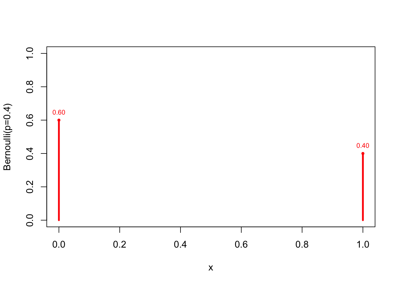
Let’s plot the Bernoulli(\(p=0.4\)) probability mass function:

plot(x=0:1, dbinom(0:1, size=1, p=0.4), 
     type ="h", lwd=3, col="red", xlab="x", 
     ylab="Bernoulli(p=0.4)", ylim=c(0,1))
points(0:1, dbinom(0:1, size=1, p=0.4), 
       pch=16, cex=0.7, col="red")
text(0:1, dbinom(0:1, size=1, p=0.4), 
     pos=3, cex=0.7, col="red", 
     labels = format(round(dbinom(0:1, size=1, p=0.4),2), nsmall=2)
     )

A sample of size 3 from the \(Bernoulli(p=0.4)\) distribution could look as follows:

set.seed(1234)
rbinom(n=3, size=1, prob=0.4)

## [1] 0 1 1

The probability of observing this sample is equal to

\[\begin{align} P(X_1=0,X_2=1, X_3=1) &\overset{ind.}{=} P(X_1=0)P(X_2=1)P(X_3=1) \\ &\overset{id.}{=} P(X=0)P(X=1)P(X=1) \\ &= (1-p)p^2 \\ &=0.6*0.4^2 \\ &=0.096. \end{align}\]

1.2 Categorical and Multinomial(\(p_1, \ldots, p_k\))

The Bernoulli distribution can handle situation where the random variable \(X\) takes on only two values, 0 and 1. These values can stand for yes/no, success/faillure or unemployed/not unemployed. Sometimes more than two categories are required. For instance, suppose that we are interested in the distribution of the following random variable:

\[\begin{align} f_X(x) &= \begin{cases} p_1 \mbox{ if person goes to work by car (x=1)} \\ p_2 \mbox{ if person goes to work by public transport (x=2)} \\ p_3 \mbox{ if person goes to work walking (x=3)} \end{cases} \\ &= p_1^{I(x=1)} p_2^{I(x=2)} p_3^{I(x=3)}, \end{align}\]

where the indicator-function \(I(x=j)\) equals 1 if \(x=j\) and zero otherwise. The parameter \(p_1\) stands for the fraction of people in the population that goes to work by car. Obviously, \(p_1+p_2+p_3=1\).

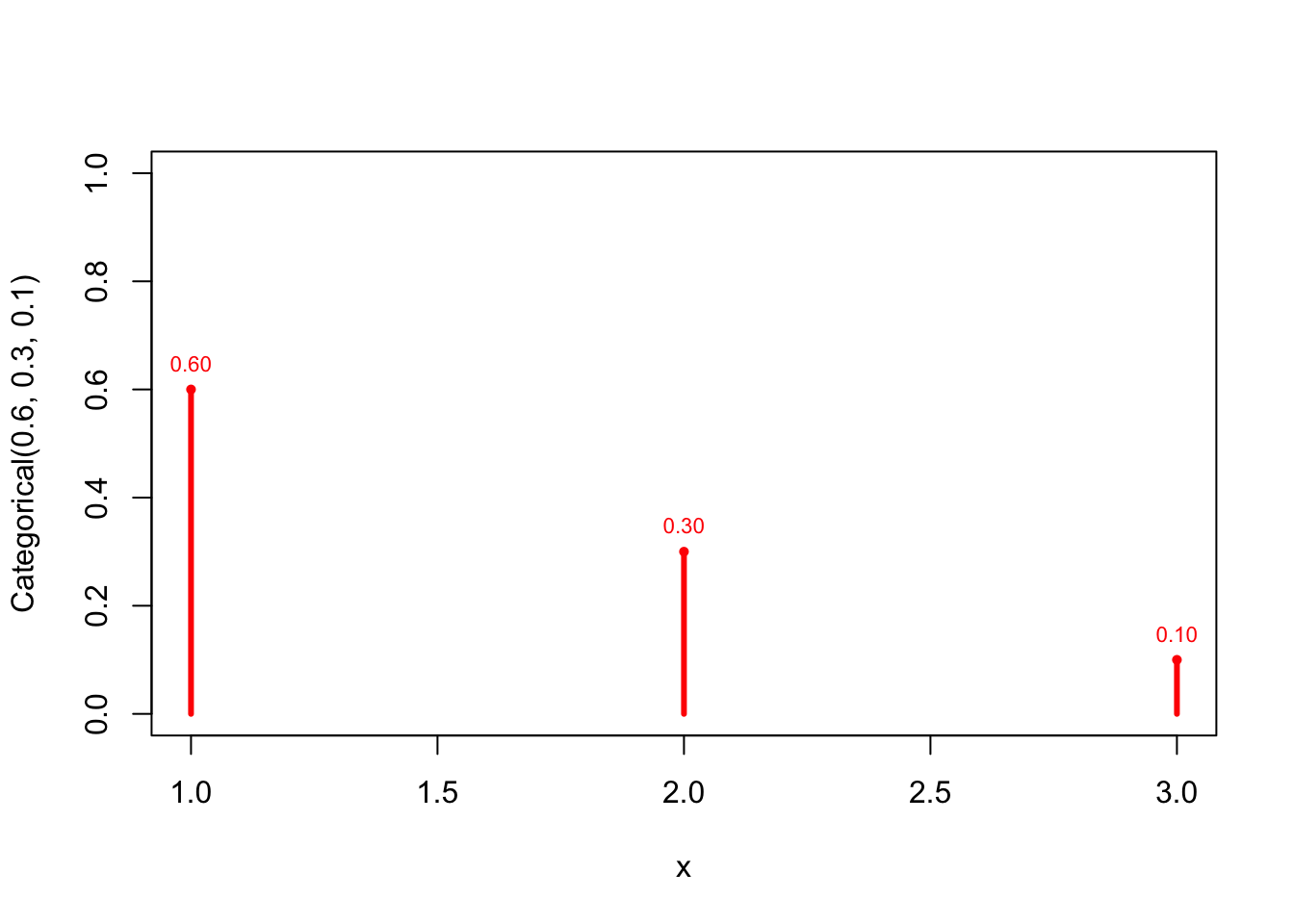
The probability mass function of the Categoricall(\(p_1=0.6,p_2=0.3,p_3=0.1\)) distribution has the following graph:

x <- 1:3
prob <- c(0.6,0.3,0.1)
plot(x=x, prob, type ="h", lwd=3, col="red", xlab="x", 
     ylab="Categorical(0.6, 0.3, 0.1)", ylim=c(0,1))
points(x, prob, pch=16, cex=0.7, col="red")
text(x, prob, pos=3, cex=0.7, col="red", 
     labels = format(round(prob,2), nsmall=2)
     )

A random sample of size \(n=10\) from the Categorical(\(0.6, 0.3, 0.1\)) distribution:

set.seed(1234)
rmultinom(n=10, size=1, prob=c(0.6,0.3,0.1))

##      [,1] [,2] [,3] [,4] [,5] [,6] [,7] [,8] [,9] [,10]
## [1,]    1    0    0    0    1    0    0    1    0     0
## [2,]    0    1    0    1    0    1    1    0    1     1
## [3,]    0    0    1    0    0    0    0    0    0     0

The first draw is from category \(1\), the second from category \(2\), up and until the tenth draw, which is from category \(2\).

The Categorical distribution is a special case of the Multinomial distribution, in that it gives the probabilities of potential outcomes of a single drawing rather than multiple drawings. That is, if \(size>1\) in the rmultinom command above, we obtain 10 draws from the Multinomial distribution:

set.seed(1234)
rmultinom(n=10, size=2, prob=c(0.6,0.3,0.1))

##      [,1] [,2] [,3] [,4] [,5] [,6] [,7] [,8] [,9] [,10]
## [1,]    2    1    1    1    2    1    1    2    0     1
## [2,]    0    1    0    1    0    1    1    0    2     1
## [3,]    0    0    1    0    0    0    0    0    0     0

1.3 Discrete Uniform(\(x_1, \ldots , x_k\))

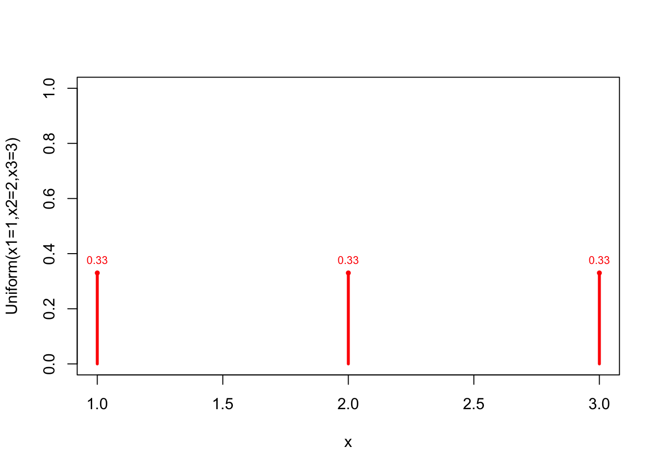
The discrete uniform distribution is a special case of the Categorical(\(p_1,\dots,p_k\)) distribution: it has \(p_1=p_2=\cdots=p_k\). With \(k=3\) and \(x_1=1,x_2=2,x_3=3\), we obtain

x <- 1:3
prob <- c(0.33,0.33,0.33)
plot(x=x, prob, type ="h", lwd=3, col="red", xlab="x", 
     ylab="Uniform(x1=1,x2=2,x3=3)", ylim=c(0,1))
points(x, prob, pch=16, cex=0.7, col="red")
text(x, prob, pos=3, cex=0.7, col="red", 
     labels = format(round(prob,2), nsmall=2)
     )

Assuming that the population distribution is Uniform(\(\{1,2,3\}\)) implies that you claim to know the population distribution: there are no unknown parameters to estimate. The mean and variance can be calculated in the usual way.

A random sample of size \(10\) from the Uniform({2,3,4,5,6}) distribution is:

library(purrr)
set.seed(1234)
rdunif(n=10, a=2, b=6)

##  [1] 5 3 6 5 2 6 5 3 3 5

1.4 Poisson(\(\lambda\))

The Poisson distribution is often used as a model for variables that represent counts. For instance, the number of custumers that have arrived in a post-office between opening and mid-day. Another example is the number of visits a person has made to his/her general practitioner during the past calendar year. A Poisson distributed random variable takes integer values, starting from zero until infinity. The values of these probabilities depend on a parameter, that is usually called \(\lambda\) (lambda), in the following way:

\[ f_X(x)= e^{- \lambda }\frac{\lambda^x}{x!} \;\;\; \lambda>0 \;\; x=0,1,\ldots. \]

The animation below shows the Poisson distributions for 19 values of \(\lambda\) between 1 and 10:

If \(X \sim Poisson(\lambda)\) then \(E[X]=\lambda\) and \(Var[X]=\lambda\). Using the animation, you can check that both the mean and the variance indeed increase with increasing values of \(\lambda\).

• Note that the family of Bernoulli distributions and the family of Multinomial distributions are not putting any restrictions on the probabilities of the population distribution. The Discrete Uniform distribution, on the other hand, makes the extreme assumption that the probabilities of the population distribution are completely known.
• The family of Poisson distributions can have many different shapes, depending on the value of the parameter \(\lambda\), but not all possible shapes. For instance, a bi-modal population distribution can never a member of the family of Poisson distributions. Therefore, assuming that the population distribution is Poisson is an assumption that may not be true. In other words, the Poisson assumption is restrictive. To give another example: there clearly exist population distributions that have a mean and a variance that are not equal to each other. These distributions cannot be a member of the Poisson family of distributions.

A random sample of size \(20\) from the Poisson(\(\lambda=1\)) distribution is:

set.seed(1234)
rpois(n=20, lambda=1)

##  [1] 0 1 1 1 2 1 0 0 1 1 1 1 0 3 0 2 0 0 0 0

2.1 N(\(\mu,\sigma^2\))

The Normal distribution with mean \(\mu\) and variance \(\sigma^2\) is denoted by \(N(\mu,\sigma^2)\). Its probability density function has the bell-curve shape. This shape is described by the pdf (for fixed values of \(\mu\) and \(\sigma^2\):

\[ f_X(x) = \frac{1}{\sigma \sqrt{2 \pi}}e^{-\frac{1}{2 \sigma^2}(x-\mu)^2}. \]

The graphic below shows the pdf, cdf and quantile function (the inverse function of the cdf) for the Normal distribution with mean \(\mu=0\) and several values of \(\sigma^2\):

As expected, the higher the value of the variance, the more the values are spread out around the mean \(\mu\). The so-called emperical rule is more specific:

If \(X \sim N(\mu,\sigma^2)\), then (approximately):

• \(P(\mu -\sigma < X < \mu + \sigma) = 0.68\)
• \(P(\mu -2\sigma < X < \mu + 2\sigma) = 0.95\)
• \(P(\mu -3\sigma < X < \mu + 3\sigma) = 0.99\)

Hence, if \(\mu=0\) and \(\sigma = 1\) \(P(-1 < X < 1)= 68\%\) and if \(\mu=0\) and \(\sigma^2=4\) \(P(-2 < X < 2)=68\%\). You can check this (and the other results) using the slider. Moreover, if \(X \sim N(\mu=0, \sigma^2=4)\), we can see that the value of \(P(X<1)\) is more or less \(0.69\) and that the \(60\%\) quantile is around \(0.51\).

We can also calculate these results ourselves:

pnorm(1, mean=0, sd=1) - pnorm(-1, mean=0, sd=1)

## [1] 0.6826895

pnorm(2, mean=0, sd=2) - pnorm(-2, mean=0, sd=2)

## [1] 0.6826895

pnorm(1, mean=0, sd=2)

## [1] 0.6914625

qnorm(0.6, mean=0, sd=2)

## [1] 0.5066942

A random sample of size \(15\) from the N(\(\mu=10, \sigma^2=9\)) distribution is:

set.seed(1234)
rnorm(n=15, mean=10, sd=3)

##  [1]  6.378803 10.832288 13.253324  2.962907 11.287374 11.518168  8.275780
##  [8]  8.360104  8.306644  7.329887  8.568422  7.004841  7.671238 10.193376
## [15] 12.878482

2.2 Exp(\(\lambda\))

The Exponential distribution is often used to model the time it takes until a certain event happens (sometimes called the survival time). The event can for instance be “someone entering the post offfice” or “the television stops working.”

The probability density function of an exponentially distributed random variable with parameter \(\lambda\) (which is sometimes called the rate) is:

\[ f_X(x) = \lambda e^{-\lambda x} \;\;\;\;\; x>0, \lambda>0. \] The pdf takes the value 0 for \(x \leq 0\). The cumulative distribution is:

\[ F_X(x) = 1 - e^{-\lambda x} \;\;\;\;\; x>0, \lambda>0. \]

We can check this:

\[\begin{align} F_X(x) &= P(X \leq x) = \int_{-\infty}^{x} f_X(t) dt = \int_{0}^{x}\lambda e^{-\lambda t} dt \\ &= \left[ -e^{-\lambda t}\right]_0^{x} = -e^{-\lambda x} - (-1) = 1 - e^{-\lambda x}. \end{align}\]

The cdf (obviously) also takes the value 0 for \(x \leq 0\). If \(X \sim Exp(\lambda)\) we have that \(E[X]=\frac{1}{\lambda}\) and \(Var[X]=\frac{1}{\lambda^2}\).

We can plot the pdf, cdf and quantile functions for different values of \(\lambda\):

The mean and variance decrease if the value of the rate \(\lambda\) increases.

A random sample of size \(10\) from the Exp(\(\lambda=1\)) distribution is:

set.seed(1234)
rexp(n=10, rate=1)

##  [1] 2.501758605 0.246758883 0.006581957 1.742746090 0.387182584 0.089949671
##  [7] 0.824081515 0.202617901 0.838040319 0.760430301

2.3 Uniform(\(a,b\))

The continuous Uniform(\(a,b\)) distribution is the continuous analog of the Discrete Uniform distribution: it takes all the real numbers between \(a\) and \(b\) as values, each of them equally likely:

\[ f_X(x) = \frac{1}{b-a} \;\;\;\; a<x<b. \] The pdf takes the value 0 for \(x \leq a\) and \(x\geq b\). The mean of a Uniform(\(a,b\)) distribution is \(\frac{1}{2}(a + b)\) and the variance is \(\frac{1}{12}(b-a)^2\).

We can easily calulate the cumulative distribution function because of the simplicity of the pdf (and hence the integrals):

\[\begin{align} F_X(x) &= \int_{a}^{x} f_X(t) dt = \int_{a}^{x} \frac{1}{b-a}dt = \left[ \frac{t}{b-a} \right]_{a}^{x} \\ &= \frac{x-a}{b-a}=-\left( \frac{a}{b-a}\right) + \left( \frac{1}{b-a} \right)x. \end{align}\]

For instance, the standard Uniform distribution (\(a=0\) and \(b=1\)) has \(F_X(x)=x\) for \(0<x<1\). The value of \(F_X(x)\) is zero for \(x<0\) and 1 for \(x>1\).

We plot the pdf, cdf and quantile function for \(a=0\) and various values of \(b\):

A random sample of size \(10\) from the Uniform(\(a=0,b=2\)) distribution is:

set.seed(1234)
runif(n=10, min=0, max=2)

##  [1] 0.22740682 1.24459881 1.21854947 1.24675888 1.72183077 1.28062121
##  [7] 0.01899151 0.46510101 1.33216752 1.02850228