4. Random Vectors
1 The General Case: Joint cdf
Multivariate random variable: A \(k-\) dimensional random variable (or: random vector) is a function with domain \(\mathbf{S}\) and codomain \(\mathbb{R}^{k}:\) \[ \left( X_{1},\ldots ,X_{k}\right) :s\in \mathbf{S}\rightarrow \left( X_{1}(s),\ldots ,X_{k}(s)\right) \in \mathbb{R}^{k}\; \text{.}\; \] The function \(\left( X_{1}(s),\ldots ,X_{k}(s)\right)\) is usually written for simplicity as \(\left( X_{1},\ldots ,X_{k}\right) \; \text{.}\;\)
Remark: If \(k=2\) we have the bivariate random variable or two dimensional random variable \[ \left( X,Y\right) :s\in \mathbf{S}\rightarrow \left( X(s),Y(s)\right) \in \mathbb{R}^{2}\; \text{.}\; \]
Joint cumulative distribution function: Let \(\left( X,Y\right)\) be a bivariate random variable. The real function of two real variables with domain \(\mathbb{R}^{2}\) and defined by \[ F_{X,Y}(x,y)=P(X\leq x,Y\leq y) \] is the joint cumulative distribution function of the two dimensional random variable \((X,Y)\; \text{.}\;\)
Example 1.1 Random Experiment: Roll two different dice (one red and one green) and write down the number of dots on the upper face of each die.
Random vector: \((X_{red},X_{green})\), where \(X_i\) is the of dots the \(i\) die, with \(i=\) green or red.
Some probabilities: \[ \begin{aligned} &P(X_{red}=2,X_{green}=4)=\frac{1}{36}\\ &P(X_{red}+X_{green}>10)=\frac{1}{12}\\ &P\left(\frac{X_{red}}{X_{green}}\leq 2\right)=P\left(\frac{X_{red}}{X_{green}}= 1\right)+P\left(\frac{X_{red}}{X_{green}}= 2\right)\\ &~~~~~~~~~~~~~~~~~~~~~=\frac{6}{36}+\frac{3}{36}=\frac{1}{4}\end{aligned} \]
Example 1.2 Random experiment: Two different and fair coins are tossed once.
Random vector: \((X_1,X_2)\), where \(X_i\) represents the number of heads obtained with coin \(i\), with \(i=1,2\).
Some probabilities: \[ \begin{aligned} P(X_1=0,X_2=0)&=P(X_1=0,X_2=1)=P(X_1=1,X_2=0)\\ &=P(X_1=1,X_2=1)=\frac{1}{4}\\ P(X_1+X_2\geq 1)&=\frac{3}{4} \end{aligned} \]
Properties of the joint cumulative distribution function:
\(0 \leq F_{X ,Y} (x ,y) \leq 1\)
\(F_{X ,Y} (x ,y)\) is non decreasing with respect to \(x\) and \(y :\)
\(\Delta _{x} >0 \Rightarrow F_{X ,Y} (x + \Delta x ,y) \geq F_{X ,Y} (x ,y)\)
\(\Delta _{y} >0 \Rightarrow F_{X ,Y} (x ,y + \Delta y) \geq F_{X ,Y} (x ,y)\)
\(\underset{x \rightarrow -\infty }{\lim }F_{X ,Y} (x ,y) =0\), \(\underset{y \rightarrow -\infty }{\lim }F_{X ,Y} (x ,y) =0\) and
\(\lim\limits_{x\to+\infty,y\to+\infty} F_{X ,Y} (x ,y) =1\)
\(P (x_{1} <X \leq x_{2} ,y_{1} <Y \leq y_{2}) =F_{X ,Y} (x_{2} ,y_{2}) -F_{X ,Y} (x_{1} ,y_{2}) -F_{X ,Y} (x_{2} ,y_{1}) +F_{X ,Y} (x_{1} ,y_{1})\text{.}\)
\(F_{X,Y}(x,y)\) is right continuous with respect to \(x\) and \(y\): \(\underset{x\rightarrow a^{+}}{\lim }F_{X,Y}(x,y)=F_{X,Y}(a,y)\) and \(\underset {y\rightarrow b^{+}}{\lim }F_{X,Y}(x,y)=F_{X,Y}(x,b)\text{.}\)
Example 1.3 Random experiment: Two different and fair coins are tossed once.
Random vector: \((X_1,X_2)\), where \(X_i\) represents the number of heads obtained with coin \(i\), with \(i=1,2\).
Joint cumulative distribution function: \[ F_{X_1,X_2}(x_1,x_2)=P(X_1\leq x_1,X_2\leq x_2)= \begin{cases} 0,& x_1<0\\ 0,& x_2<0\\ \frac{1}{4},&0\leq x_1<1,0\leq x_2<1\\ \frac{1}{2},&0\leq x_1<1,x_2\geq 1\\ \frac{1}{2},&0\leq x_2<1,0\leq x_1<1\\ 1,&x_1\geq 1,x_2\geq 1 \end{cases} \]
2 The General Case: Marginal cdf
The (marginal) cumulative distribution functions of \(X\) and \(Y\) can be obtained form the Joint cumulative distribution functions of \(\left( X,Y\right) :\)
The Marginal cumulative distribution function of \(X:\) \(F_{X}(x)=P\left( X\leq x\right) =P\left( X\leq x,Y\leq +\infty \right) = \underset{y\rightarrow +\infty }{\lim }F_{X,Y}(x,y)\text{.}\)
The Marginal cumulative distribution function of \(Y:\) \(F_{Y}(y)=\left( Y\leq y\right) =P\left( X\leq +\infty ,Y\leq y\right) = \underset{x\rightarrow +\infty }{\lim }F_{X,Y}(x,y)\text{.}\)
Remark: The joint distribution uniquely determines the marginal distributions, but the inverse is not true.
Example 2.1 Random experiment: Two different and fair coins are tossed once.
Random vector: \((X_1,X_2)\), where \(X_i\) represents the number of heads obtained with coin \(i\), with \(i=1,2\).
Joint cululative distribution function: \[ F_{X_1,X_2}(x_1,x_2)=\begin{cases} 0,& x_1<0\text{ or } x_2<0\\ \frac{1}{4},&0\leq x_1<1,0\leq x_2<1\\ \frac{1}{2},&0\leq x_1<1,x_2\geq 1\\ \frac{1}{2},&0\leq x_2<1,0\leq x_1<1\\ 1,&x_1\geq 1,x_2\geq 1 \end{cases} \] Marginal cumulative distribution function for \(X_1\): \[ F_{X_1}(x_1)=\lim_{x_2\to+\infty} F_{X_1,X_2}(x_1,x_2)=\begin{cases} 0,& x_1<0\\ \frac{1}{2},&0\leq x_1<1\\ 1,&x_1\geq 1 \end{cases} \]
Example 2.2 Let \((X,Y)\) be a jointly distributed random variable with CDF: \[ F_{X,Y}(x,y)=\begin{cases} 1-e^{-x}-e^{-y}+e^{-x-y},&x\geq 0, y\geq 0\\ 0,&x<0,y<0 \end{cases}. \] Marginal cumulative distribution function of the random variable \(X\) is: \[ F_{X}(x)=\begin{cases} 1-e^{-x},&x\geq 0\\ 0,&x<0 \end{cases}. \]
Marginal cumulative distribution function of the random variable Y is: \[ F_{Y}(y)=\begin{cases} 1-e^{-y},&y\geq 0\\ 0,&y<0 \end{cases}. \]
3 The General Case: Independence
Definition: The jointly distributed random variables \(X\) and \(Y\) are said to be independent if and only if for any two sets \(B_{1}\in \mathbb{R},\) \(B_{2}\in \mathbb{R}\) we have \[ P(X\in B_{1},Y\in B_{2})=P(X\in B_{1})P(Y\in B_{2}) \]
Remark: Independence implies that \(F_{X,Y}(x,y)=F_{X}(x)F_{Y}(y)\text{,}\) for any \(\left( x,y\right) \in \mathbb{R}^{2}\text{.}\)
Theorem: If \(X\) and \(Y\) are independent random variables and if \(h(X)\) and \(g(Y)\) are two functions of \(X\) and \(Y\) respectively, then the random variables \(U=h(X)\) and \(V=g(Y)\) are also independent random variables.
Example 3.1 Random experiment: Two different and fair coins are tossed once.
Random vector: \((X_1,X_2)\), where \(X_i\) represents the number of heads obtained with coin \(i\), with \(i=1,2\).
Are these random variables independent? \[ F_{X_1}(x_1)= \begin{cases} 0,& x_1<0\\ \frac{1}{2},&0\leq x_1<1\\ 1,&x_1\geq 1 \end{cases}, \quad F_{X_2}(x_2)= \begin{cases} 0,& x_2<0\\ \frac{1}{2},&0\leq x_2<1\\ 1,&x_2\geq 1 \end{cases} \]
One can easily verify that \(F_{X_1,X_2}(x_1,x_2)=F_{X_1}(x_1)\times F_{X_1}(x_1)\). \[ F_{X_1,X_2}(x_1,x_2)= \begin{cases} 0,& x_1<0\text{ or } x_2<0\\ \frac{1}{4},&0\leq x_1<1,0\leq x_2<1\\ \frac{1}{2},&0\leq x_1<1,x_2\geq 1\\ \frac{1}{2},&0\leq x_2<1,0\leq x_1<1\\ 1,&x_1\geq 1,x_2\geq 1 \end{cases} \]
Example 3.2 Let \((X,Y)\) be a jointly distributed random variable with CDF: \[ F_{X,Y}(x,y)=\begin{cases} 1-e^{-x}-e^{-y}+e^{-x-y},&x\geq 0, y\geq 0\\ 0,&x<0,y<0 \end{cases}. \] Marginal cumulative distribution function of the random variable \(X\) and \(Y\) are: \[ \begin{aligned} &F_{X}(x)=\lim_{y\to+\infty}F_{X,Y}(x,y)=\begin{cases} 1-e^{-x},&x\geq 0\\ 0,&x<0 \end{cases}\\ &F_{Y}(y)=\lim_{x\to+\infty}F_{X,Y}(x,y)=\begin{cases} 1-e^{-y},&y\geq 0\\ 0,&y<0 \end{cases}. \end{aligned} \]
\(X\) and \(Y\) are independent random variables because: \[ F_{X,Y}(x,y)=F_{X}(x)F_Y(y) \]
since \[ 1-e^{-x}-e^{-y}+e^{-x-y}=(1-e^{-y})(1-e^{-x}). \]
4 Discrete Random Variables
4.1 Joint pmf
Let \(D_{(X,Y)}\) be the set of of discontinuities of the joint cumulative distribution function \(F_{(X,Y)}(x,y)\text{,}\) that is \[ D_{(X,Y)}=\left \{ \left( x,y\right) \in \mathbb{R}^{2}:P(X=x,Y=y)>0\right \} \]
Definition: \((X,Y)\) is a two dimensional discrete random variable if and only if \[ \sum_{\left( x,y\right) \in D_{(X,Y)}}P\left( X=x,Y=y\right) =1. \]
Remark: As in the univariate case, a multivariate discrete random variable can take a finite number of possible values \((x_{i},y_{j}),\) where \(i=1,2,...,k_{1}\text{ and }j=1,2,...,k_{2}\text{,}\) where \(k_{1}\) and \(k_{2}\) are finite integers, or a countably infinite \((x_{i},y_{j}),\) where \(i=1,2,...\) and \(j=1,2,...\). For the sake of generality we consider the latter case. That is \(D_{(X,Y)}=\left \{ (x_{i},y_{j}),i=1,2,...,j=1,2,...\right \}\)
Joint probability mass function: If \(X\) and \(Y\) are discrete random variables, then the function given by \[ f_{X,Y}(x,y)=P\left( X=x,Y=y\right) \] for \((x,y)\in D_{(X,Y)}\) is called the joint probability mass function of \((X,Y)\) (joint pmf) or joint probability distribution of the random variables \(X\) and \(Y\text{.}\)
Theorem: A bivariate function \(f_{X,Y}(x,y)\) can serve as joint probability mass function of the pair of discrete random variables \(X\) and \(Y\) if and only if its values satisfy the conditions:
\(f_{X,Y}(x,y)\geq 0\) for any \((x,y)\in \mathbb{R}^{2}\)
\(\sum _{\left (x ,y\right ) \in D_{(X ,Y)}}f_{X ,Y} (x ,y) =\sum _{i =1}^{\infty }\sum _{j =1}^{\infty }f_{X ,Y} (x_{i} ,y_{j}) =1\)
Remark: We can calculate any probability using this function. For instance \(P\left( \left( x,y\right) \in B\right) =\sum_{\left( x,y\right) \in B}f_{X,Y}(x,y)\)
Example 4.1 Let \(X\) and \(Y\) be the random variables representing the population of monthly wages of husbands and wives in a particular community. Say, there are only three possible monthly wages in euros: \(0\), \(1000\), \(2000\). The joint probability mass function is
| \(\mathbf{X=0}\) | \(\mathbf{X=1000}\) | \(\mathbf{X=2000}\) | |
|---|---|---|---|
| \(\mathbf{Y=0}\) | \(0.05\) | \(0.15\) | \(0.10\) |
| \(\mathbf{Y=1000}\) | \(0.10\) | \(0.10\) | \(0.30\) |
| \(\mathbf{Y=2000}\) | \(0.05\) | \(0.05\) | \(0.10\) |
The probability that a husband earns \(2000\) euros and the wife earns \(1000\) euros is given by \[\begin{aligned} f_{X,Y}(2000,1000) &=P(X=2000,Y=1000) \\ &=0.30\end{aligned}\]
4.2 Joint cdf
Joint cumulative distribution function: If \(X\) and \(Y\) are discrete random variables, the function given by \[ F_{X,Y}(x\;y)=\sum_{s\leq x}\sum_{t\leq y}f_{X,Y}(s,t) \] for \(\left( x,y\right) \in \mathbb{R}^{2}\) is called the joint distribution function or joint cumulative distribution of \(X\) and \(Y\text{.}\)
4.3 Marginal pmf’s
Marginal probability distribution/function: If \(Y\) and \(X\) are discrete random variables and \(f_{X,Y}\) is the value of their joint probability distribution at \((x,y)\) the function given by
\[ \begin{aligned} P\left( X=x\right) &=&\left \{ \begin{array}{cc} \sum_{y\in D_{y}}f(x,y)=\sum_{y\in D_Y}f_{X,Y}(x,y), & \; \text{for}\;x\in D_{x} \\ 0, & \; \text{for}\;x\notin D_{x} \end{array} \right. \; \text{.}\; \\ P\left( Y=y\right) &=&\left \{ \begin{array}{cc} \sum_{x\in D_{x}}f(x,y)=\sum_{x\in D_X}f_{X,Y}(x,y), \; \; & \; \text{for}\;y\in D_{y} \\ 0, & \; \text{for}\;y\notin D_{y} \end{array} \right. \end{aligned} \]
are respectively is the Marginal probability distribution of the r.v. \(X\) and \(Y\), where \(D_{x}\) and \(D_{y}\) are the range of \(X\) and \(Y\) respectively.
Example 4.2 \[ \begin{aligned} P\left( X=x\right) =&P\left( X=x,Y=0\right) +P\left( X=x,Y=1000\right) \\ &+P\left( X=x,Y=2000\right) \\ P\left( Y=y\right) =&P\left( X=0,Y=y\right) +P\left( X=1000,Y=y\right) \\ &+P\left( X=2000,Y=y\right) \end{aligned} \]
Applying these formulas we have:
| \(\mathbf{X=0}\) | \(\mathbf{X=1000}\) | \(\mathbf{X=2000}\) | \(f_Y(y)\) | |
|---|---|---|---|---|
| \(\mathbf{Y=0}\) | \(0.05\) | \(0.15\) | \(0.10\) | \(0.3\) |
| \(\mathbf{Y=1000}\) | \(0.10\) | \(0.10\) | \(0.30\) | \(0.5\) |
| \(\mathbf{Y=2000}\) | \(0.05\) | \(0.05\) | \(0.10\) | \(0.2\) |
| \(f_X(x)\) | \(0.2\) | \(0.3\) | \(0.5\) | \(1\) |
\[ \begin{aligned} &F_{X,Y}(1000,1000)=P(X=0,Y=0)+P(X=0,Y=1000) \\ &~~~~~~~~~~~~~+P(X=1000,Y=0)+P(X=1000,Y=1000)\\ &F_{X,Y}(0,1000)=P(X=0,Y=0)+P(X=0,Y=1000) \end{aligned} \]
4.4 Independence
Independence of random variables: Two discrete random variables \(X\) and \(Y\) are independent if and only if, for all \((x,y)\in D_{X,Y}\), \[ P\left( X=x,Y=y\right) =P\left( X=x\right) P\left( Y=y\right) \text{.} \]
| \(\mathbf{X=0}\) | \(\mathbf{X=1000}\) | \(\mathbf{X=2000}\) | \(f_Y(y)\) | |
|---|---|---|---|---|
| \(\mathbf{Y=0}\) | \(0.05\) | \(0.15\) | \(0.10\) | \(0.3\) |
| \(\mathbf{Y=1000}\) | \(0.10\) | \(0.10\) | \(0.30\) | \(0.5\) |
| \(\mathbf{Y=2000}\) | \(0.05\) | \(0.05\) | \(0.10\) | \(0.2\) |
| \(f_X(x)\) | \(0.2\) | \(0.3\) | \(0.5\) | \(1\) |
Are these two random variables independent?
\[ \begin{aligned} &P(X=2000,Y=2000)=P(X=2000)\times P(Y=2000)=0.1\\ &\text{Is this sufficient to say that }X\text{ and }Y\text{ are independent?}\textbf{ NO!}\\ &P(X=0,Y=0)=0.05\text{ but }P(X=0)P(Y=0)=0.06\end{aligned} \] thus \(X\) and \(Y\) are not independent.
4.5 Conditional pmf’s
Conditional probability mass function of \(Y\) given \(X\):A conditional probability function of a discrete random variable \(Y\) given another discrete variable \(X\) taking a specific value is defined as \[\begin{aligned} f_{Y|X=x}(y) =&P\left( Y=y{|}X=x\right) =\frac{P\left( Y=y,X=x\right) }{P\left( X=x\right) } \\ =&\frac{f_{X,Y}(x,y)}{f_{X}(x)},\; \text{{}}\;f_{X}(x)>0, \text{ for a fixed $x$.}\end{aligned}\] The conditional probability function of \(X\) given \(Y\) is defined by
\[ f_{X|Y=y}(x)=\frac{f_{X,Y}(x,y)}{f_{Y}(y)},\; \text{{}}\;f_{Y}(y)>0. \]
Remarks:
The conditional probability functions satisfy all the properties of probability functions, and therefore \(\sum _{i =1}^{\infty }f_{Y\vert X} (y_{i}) =1.\)
If \(X\) and \(Y\) are independent\(f_{Y|X=x}(y)=f_{y}(y)\) and \(f_{X|Y=y}(x)=f_{X}(x)\)
example Consider the joint probability function
| \(\mathbf{X=0}\) | \(\mathbf{X=1000}\) | \(\mathbf{X=2000}\) | \(f_Y(y)\) | |
|---|---|---|---|---|
| \(\mathbf{Y=0}\) | \(0.05\) | \(0.15\) | \(0.10\) | \(0.3\) |
| \(\mathbf{Y=1000}\) | \(0.10\) | \(0.10\) | \(0.30\) | \(0.5\) |
| \(\mathbf{Y=2000}\) | \(0.05\) | \(0.05\) | \(0.10\) | \(0.2\) |
| \(f_X(x)\) | \(0.2\) | \(0.3\) | \(0.5\) | \(1\) |
Compute \(P\left( Y=y{|}X=0\right)\).
\[ \begin{aligned} P\left( Y=0{|}X=0\right) &=&\frac{P\left( Y=0,X=0\right) }{P\left( X=0\right) }=\frac{0.05}{0.2}=0.25 \\ P\left( Y=1000{|}X=0\right) &=&\frac{P\left( Y=1000,X=0\right) }{P\left( X=0\right) }=\frac{0.1}{0.2}=0.5\text{.} \\ P\left( Y=2000{|}X=0\right) &=&\frac{P\left( Y=2000,X=0\right) }{P\left( X=0\right) }=\frac{0.05}{0.2}=0.25\text{.}\end{aligned} \]
4.6 Conditional cdf’s
Definition: The conditional CDF of \(Y\) given \(X\) is defined by
\[ F_{Y\vert X=x}(y)=P\left( Y\leq y{|}X=x\right) =\sum_{y'\in D_Y\wedge y'\leq y}\frac{P\left( Y=y',X=x\right) }{P\left( X=x\right) } \] for a fixed \(x\), with \(P(X=x)>0\).
Remark: It can be checked that \(F_{Y\vert X=x}\) is indeed a CDF.
Exercice: Verify that \(F_{Y\vert X=x}\) is non-decreasing and and \(\lim\limits_{y\to+\infty}F_{Y\vert X=x}(y)=1\).
\[ \begin{aligned} 1)~~F_{Y\vert X=x}&(y+\delta)-F_{Y\vert X=x}(y)\\ &~~~~~~~~~~~=\frac{P\left( Y\leq y+\delta,X=x\right)}{P(X=x)}-\frac{P\left( Y\leq y,X=x\right)}{P(X=x)}\geq 0.\\ 2)~~~\lim_{y\to+\infty}&F_{Y\vert X=x}(y)=\lim_{y\to+\infty}P\left( Y\leq y\vert X=x\right)\\ =\lim_{y\to+\infty}&\frac{P\left( Y\leq y,X=x\right)}{P\left( X=x\right)}=\frac{P\left( Y\leq \infty,X=x\right)}{P\left( X=x\right)}=\frac{P\left(X=x\right)}{P\left( X=x\right)}=1. \end{aligned} \]
Example 4.3 Consider the conditional probability of \(Y\) given that \(X=0\) previously deduced: \[ \begin{aligned} P\left( Y=0{|}X=0\right) &=\frac{P\left( Y=0,X=0\right) }{P\left( X=0\right) }=\frac{0.05}{0.2}=0.25 \\ P\left( Y=1000{|}X=0\right) &=\frac{P\left( Y=1000,X=0\right) }{P\left( X=0\right) }=\frac{0.1}{0.2}=0.5\text{.} \\ P\left( Y=2000{|}X=0\right) &=\frac{P\left( Y=2000,X=0\right) }{P\left( X=0\right) }=\frac{0.05}{0.2}=0.25\text{.} \end{aligned} \]
Then the conditional CDF of \(Y\) given that \(X=0\) is
\[ F_{Y\vert X=0}(y)= \begin{cases} 0,&y<0\\ 0.25,&0\leq y<1000\\ 0.75,&1000\leq y<2000\\ 1,&y\geq 0 \end{cases}. \]
5 Continuous Random Variables
5.1 Joint pdf and joint cdf
Definition: \(\left( X,Y\right)\) is a two-dimensional continuous random variable with a joint cumulative distribution function \(F_{X,Y}(x,y)\text{,}\) if and only if \(X\) and \(Y\) are continuous random variables and there is a non-negative real function \(f_{X,Y}(x,y)\text{,}\) such that \[ F_{X,Y}(x,y)=P(X\leq x,Y\leq y)=\int_{-\infty }^{y}\int_{-\infty }^{x}f_{X,Y}(t,s)dtds. \]
The function \(f_{X,Y}(x,y)\) is the joint (probability) density of \(X\) and \(Y\).
Remark: Let \(A\) be a set in the \(\mathbb{R}^2\). Then, \[ P\left((X,Y)\in A\right)=\int\int_{A}f_{X,Y}(t,s)dtds. \]
::: {.example} Joint probability density function of the two dimensional random variable \((P_1,S)\) where \(P_1\) represents the price and \(S\) the total sales (in 10000 units).
Joint probability density function: \[ f_{P_1,S}(p,s)=\begin{cases} 5pe^{-ps},& 0.2<p<0.4,~~s>0\\ 0,& \text{otherwise} \end{cases} \]
Joint cumulative distribution function: \[\begin{aligned} F_{P_1,S}(p,s)&=P(P_1\leq p,S\leq s)\\ &=\begin{cases} 0,&p<0.2 \text{ or }s<0\\ -1+5p-5\frac{e^{-0.2s}-e^{-ps}}{s},& 0.2<p<0.4, s\geq 0\\ 1-5\frac{e^{-0.2s}-e^{-0.4s}}{s},& p\geq 0.4, s\geq 0 \end{cases} \end{aligned} \] To get the CDF we need to make the following computations:
If \(p<0.2 \text{ or }s<0\), then \(f_{P_1,S}(p,s)=0\) and \[ \begin{aligned} P(P_1\leq p,S\leq s)=\int_{-\infty}^p\int_{-\infty}^sf_{P_1,S}(t,u)dtdu=0 \end{aligned} \]
If \(0.2<p<0.4\) and \(s\geq 0\), then \[ \begin{aligned} &P(P_1\leq p,S\leq s)=\int_{-\infty}^p\int_{-\infty}^sf_{P_1,S}(t,u)dtdu\\ &~~~~~~~~=\int_{0.2}^p\int_{0}^sf_{P_1,S}(t,u)dtdu= -1+5p-5\frac{e^{-0.2s}-e^{-ps}}{s} \end{aligned} \]
If \(p\geq 0.4\) and \(s\geq 0\), then \[ \begin{aligned} &P(P_1\leq p,S\leq s)=\int_{-\infty}^p\int_{-\infty}^sf_{P_1,S}(t,u)dtdu\\ &~~~~~~~~=\int_{0.2}^{0.4}\int_{0}^sf_{P_1,S}(t,u)dtdu= 1-5\frac{e^{-0.2s}-e^{-0.4s}}{s} \end{aligned} \]
Theorem: A bivariate function can serve as a joint probability density function of a pair of continuous random variables \(X\) and \(Y\) if its values, \(f_{X,Y}(x,y)\), satisfy the conditions:
\(f_{X ,Y} (x ,y) \geq 0\text{,}\) for all \((x ,y) \in \mathbb{R}^{2}\)
\(\int _{ -\infty }^{ +\infty }\int _{ -\infty }^{ +\infty }f_{X ,Y} (x ,y) d x d y =1.\)
Property: Let \((X,Y)\) be a bivariate random variable and \(B\in\mathbb{R}^2\), then \[ P((X,Y)\in B)=\int\int_{B}f_{X,Y}(x,y)dxdy. \]
Example 5.1 Let \((X,Y)\) be a continuous bi-dimensional random variable with density function \(f_{X,Y}\) given by \[ f_{X,Y}(x,y)=\begin{cases} kx+y,&0<x<1,0<y<1\\ 0,&\text{otherwise} \end{cases}. \] Find \(k\).
Solution: From the first condition, we know that \(f_{X,Y}(x,y)\geq 0\). Therefore \(k\geq 0\). Additionally, \[ \int _{ -\infty }^{ +\infty }\int _{ -\infty }^{ +\infty }f_{X ,Y} (x ,y) d x d y =1. \] This is equivalent to \[ \int _{ 0 }^{ 1 }\int _{0 }^{ 1 }kx+y d x d y =1\Leftrightarrow\frac{1+k}{2}=1\Leftrightarrow k=1. \]
::: {.example} Let \((X,Y)\) be a continuous bi-dimensional random variable with density function \(f_{X,Y}\) given by \[ f_{X,Y}(x,y)=\begin{cases} x+y,&0<x<1,0<y<1\\ 0,&\text{otherwise} \end{cases}. \] Compute \(P(X>Y)\).
Solution: Firstly, we notice that
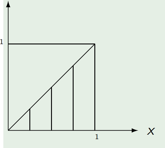
\[ \begin{aligned} P(X>Y)&=\int _{ 0 }^{ 1 }\int _{0 }^{ x }(x+y) d y d x \\ &=\int _{ 0 }^{ 1 }\frac{3}{2}x^2dx=\frac{1}{2} \end{aligned} \]
Properties: Let \((X,Y)\) be a continuous bivariate random variable. If \(f_{X,Y}\) represents the density function of \((X,Y)\) and \(F_{X,Y}\) represents respectively joint CDF of \((X,Y)\). Then,
- \(f_{X,Y}(x,y)=\frac{\partial ^{2}F_{X,Y}(x,y)}{\partial x\partial y}= \frac{\partial ^{2}F_{X,Y}(x,y)}{\partial y\partial x}\text{, almost everywhere.}\)
5.2 Marginal pdf’s
Marginal density functions of the random variable \(X\) \[ f_{X} \left (x\right ) =\int _{ -\infty }^{ +\infty }f_{X ,Y} (x ,v) d v \text{,} \]
Marginal density functions of the random variable \(Y\) \[ f_{Y}\left( y\right) =\int_{-\infty }^{+\infty }f_{X,Y}(u,y)du. \]
5.3 Marginal cdf’s
Marginal CDF of the random variable \(X\) \[ F_{X} \left (x\right ) =\underset{y \rightarrow +\infty }{\lim }F_{X ,Y} (x ,y) =\int _{ -\infty }^{x}\underbrace{\int _{ -\infty }^{ +\infty }f_{X ,Y} (u ,y) d y}_{=f_{X}(u)} d u\text{,} \]
Marginal CDF of the random variable \(Y\) \[ F_{Y}\left( y\right) =\underset{x\rightarrow +\infty }{\lim } F_{X,Y}(x,y)=\int_{-\infty }^{y}\underbrace{\int_{-\infty }^{+\infty }f_{X,Y}(x,v)dv}_{=f_Y(v)}dx \text{.} \]
Example 5.2 Joint density function: \[ f_{P,S}(p,s)=\begin{cases} 5pe^{-ps},& 0.2<p<0.4,~~s>0\\ 0,& \text{otherwise} \end{cases} \]
Marginal density function of \(P\): \[ \begin{aligned} f_P(p)&=\int_{-\infty}^{+\infty} f_{P,S}(p,s)ds=\begin{cases} 5\underbrace{\int_0^{+\infty}pe^{-ps}ds}_{=1},& 0.2<p<0.4\\ 0,& \text{otherwise} \end{cases}\\ &=\begin{cases} 5,& 0.2<p<0.4\\ 0,& \text{otherwise} \end{cases} \end{aligned} \]
Marginal cumulative distribution function: \[ \begin{aligned} F_{S}(s)&=\lim_{p\to+\infty}F_{P,S}(p,s)=\begin{cases} 0,&s<0\\ 1-5\frac{e^{-0.2s}-e^{-0.4s}}{s^2},& s\geq 0 \end{cases} \end{aligned} \]
5.4 Conditional pdf’s
Definition: If \(f_{X,Y}(x,y)\) is the joint probability density function of the continuous random variables \(X\) and \(Y\) and \(f_{Y}\left( y\right)\) is the marginal density function of \(Y\), the function given by \[ f_{X|Y=y}\left( x\right) =\frac{f_{X,Y}(x,y)}{f_{Y}\left( y\right) },x\in \mathbb{R}\; \text{ (for fixed }y \text{),}\;f_{Y}\left( y\right) > 0 \] is the conditional probability density function of \(\bf X\) given \(\left \{\bf Y=y\right \} \text{.}\) Similarly if \(f_{X}\left( x\right)\) is the marginal density function of \(X\) \[ f_{Y|X=x}\left( y\right) =\frac{f_{X,Y}(x,y)}{f_{X}\left( x\right) },y\in \mathbb{R}\; \text{(for fixed }x\text{),}\;f_{X}\left( x\right) > 0 \] is the conditional probability function of \(Y\) given \(\left \{ X=x\right \}\).
Remark: Note that \[ P\left( X\in B|Y=y\right) =\int_{B}f_{X|Y=y}\left( x\right) dx \] for any \(B\subset \mathbb{R}\).
Example 5.3 \((X,Y)\) is a random vector with the following joint density function: \[ f_{X,Y}(x,y)=\left\{ \begin{array}{cc} \left( y+x\right) & \; \text{for}\; \left( x,y\right) \in \left( 0,1 \right) \times \left( 0,1 \right) \\ 0 & \text{otherwise} \end{array} \right.. \]
Conditional density function of \(Y\) given that \(X=x\) (with \(x\in(0,1)\)):
\[ \begin{aligned} f_X(x)&=\int_0^1(y+x)dy\\ &=x+\frac{1}{2} \end{aligned} \]
\[ \begin{aligned} f_{Y|X=x}\left( y\right) &=\frac{f_{X,Y}(x,y)}{f_{X}(x)} \\ &=\frac{x+y}{x+\frac{1}{2}}, \, y\in(0,1) \end{aligned} \]
Probability of \(Y\geq 0.7|X=0.5\) \[ \begin{aligned} P(Y\geq 0.7|X=0.5)&=\int_{0.7}^{1}f_{Y|X=0.5}\left( y\right) dy\\ &=\int_{0.7}^{1}\left( y+0.5\right) dy=0.405. \end{aligned} \]
Remark:
The conditional density functions of \(X\) and \(Y\) verify all the properties of a density function of a univariate random variable.
Note that we can always decompose a joint density function in the following way \[ f_{X,Y}(x,y)=f_{X}(x)f_{Y|X=x}\left( y\right) =f_{Y}\left( y\right) f_{X|Y=y}\left( x\right) . \]
5.5 Independence
- If \(X\) and \(Y\) are independent \(f_{Y|X=x}\left( y\right) =f_{Y}\left( y\right)\) and \(f_{X|Y=y}\left( x\right) =f_{X}\left( x\right) \text{.}\)
Example 5.4 Consider the conditional density function of \(Y\) given that \(X=x\) (with \(x\in(0,1)\)): \[ \begin{aligned} f_{Y|X=x}\left( y\right) &=\frac{f_{X,Y}(x,y)}{f_{X}(x)} =\frac{x+y}{x+\frac{1}{2}}, \, y\in(0,1). \end{aligned} \]
\(f_{Y|X=x}\) is indeed a density function: \[ f_{Y|X=x}(y)\geq 0\quad\text{and}\quad\int_0^{1}\frac{x+y}{x+\frac{1}{2}}dy=1. \]
Example 5.5 Consider the conditional density function of \(Y\) given that \(X=x\) (with \(x\in(0,1)\)) and the marginal density function of \(Y\). \[ \begin{aligned} f_{Y|X=x}\left( y\right) &=\frac{f_{X,Y}(x,y)}{f_{X}(x)} =\frac{x+y}{x+\frac{1}{2}}, \, y\in(0,1)\\ f_Y(y)&=y+\frac{1}{2}, \, y\in(0,1). \end{aligned} \]
The random variables are not independent because \[ f_{Y|X=x}(y)\neq f_{Y}(y),\quad\text{for some }y\in (0,1). \]
5.6 Conditional cdf’s
Definition: The conditional CDF of \(Y\) given \(X\) by defined by \[F_{Y\vert X=x}(y)=\int_{-\infty}^yf_{Y\vert X=x}(s)ds=\int_{-\infty}^y\frac{f_{Y, X}(s,x) }{f_X(x) }ds \] for a fixed \(x\), with \(f_X(x)>0\).
Remark: It can be checked that \(F_{Y\vert X=x}\) is indeed a CDF.
Example 5.6 Consider the conditional density function of \(Y\) given that \(X=x\) (with \(x\in(0,1)\)): \[ \begin{aligned} f_{Y|X=x}\left( y\right) &=\frac{f_{X,Y}(x,y)}{f_{X}(x)} =\frac{x+y}{x+\frac{1}{2}}, \, y\in(0,1). \end{aligned} \]
For \(x\in(0,1)\), the conditional cumulative density function is given by: \[ \begin{aligned} F_{Y\vert X=x}(y)=\begin{cases} 0,&y< 0\\ \frac{y (2 x + y)}{1 + 2 x},&0\leq y<1\\ 1,& y\geq 1 \end{cases} \end{aligned} \]
where, \(\frac{y (2 x + y)}{1 + 2 x}=\int_0^{y}\frac{x+s}{x+\frac{1}{2}}ds\).