1. Probability Theory
1 Revisions: Methods of Enumeration
Multiplication Principle: If an operation consists of two steps, of which the 1st can be done in \(n_1\) ways and for each of these the 2nd one can be done in \(n_2\) ways, then the whole operation can be done in \(n_1?n_2\) ways.
If an operation consists of k steps of which the 1st can be done in \(n_1\) ways, for each of these the 2nd step can be done in \(n_2\) ways, and so forth,then the whole operation can be done in \(n_1\times n_2\times \cdots \times n_k\) ways.
Example 1.1 John, in his daily job, has 3 different tasks to complete. The first one can be done in 3 different ways, the second one in 5 different ways and the last one in 2 different ways.
Therefore, John can complete his job in \[\underbrace{~~3~~}_{T1}\times\underbrace{~~5~~}_{T2}\times\underbrace{~~2~~}_{T3}=30 \text{ different ways.}\]
Permutations: A permutation is a distinct arrangement of n different elements of a set.
Permutations (all elements are different): Suppose that \(n\) positions are to be filled with \(n\) distinct objects. There are \(n\) choices for the 1st position, \(n-1\) choices for the 2nd position, \(\cdots, 1\) choice for the last position. So by the multiplication principle, the number of possible arrangements are \[\underline{~~n~~}\times\underline{n-1}\times\underline{n-2}\times\cdots\times\underline{~~1~~}=n!\]
Example 1.2 Example: Consider the set \(\{1,2,3\}\). The possible numbers containing the 3 different digits in the set are: \(123\), \(132\), \(213\), \(231\), \(312\) and \(321\). Hence there are 3!=6 permutations.
Example 1.3 The number of permutations of the four-letters \(a,b,c,d =4!=24\)
Permutation of \(n\) distinct objects (ordered sampling is without replacement): This is \(n!\).
Filling \(r\) positions, having \(n\) objects:
Permutations Rule (when items are all different):
There are \(n\) different items available;
We select \(r\) of the \(n\) items (without replacement);
We consider rearrangements of the same items to be different sequences. For instance 123 is a different sequence from 132.
Permutation of \(n\) objects taken \(r\) at a time: If only \(r\) positions are to be filled with \(n\) distinct objects and \(r\leq n\), the number of possible ordered arrangements is \[\begin{aligned} _nP_r&=\underline{~~~n~~~}\times\underline{~n-1~}\times\cdots\times\underline{n-r+1}=\frac{n!}{(n-r)!} \end{aligned}\]
Example 1.4 At home, Mike has 4 different colored light bulbs available for two lamps. He wants to know how many different ways there are to fix the light bulbs in the lamps.
\[\begin{aligned} {_4P_2}=&\underbrace{~~4~~}_{L_1}\times\underbrace{~~3~~}_{L_2}\\=&\frac{4!}{2!}=12 \end{aligned}\]
Example 1.5 With pieces of cloth of 4 different colours how many distinct three band vertical colored-flags can one make if the colors can’t be repeated? \[_4P_3=\frac{4!}{1!}=24.\]
\[\begin{aligned} \hspace{-0.2cm}\Longrightarrow\textit{Up to now, order matters and sampling is without replacement.}\Longleftarrow \end{aligned}\]
Permutation of \(n\) distinct objects (ordered sampling with replacement) : The number of possible arrangements are \(n^n\).
\[\underline{~~n~~}\times\underline{~~n~~}\times\underline{~~n~~}\times\cdots\times\underline{~~n~~}=n^n\]
Example 1.6 The number of possible four-letters code words using \(a,b,c,d\) is \(4^4=256\).
Distinguishable Permutation: Suppose a set of n objects of r distinguishable types. From these n objects, \(k_1\) are similar, \(k_2\) are similar, \(\cdots\), \(k_r\) are similar, so that \(k_1+k_2+\cdots+k_r = n\). The number of distinguishable permutations of these n objects is: \[\frac{n!}{k_1!\times k_2!\times\cdots\times k_r!}\] which is known a Multinomial Coefficient.
Example 1.7 Exercise: With 9 balls of 3 different colours, 3 black, 4 green and 2 yellow, how many distinguishable groups can one make?
Answer: \[\frac{9!}{3!\times 4!\times 2!}=1260\]
Combinations rule (order does not matter):
There are \(n\) different items available;
We select \(r\) of the \(n\) items (without replacement);
We consider rearrangements of the same items to be the same. For instance 123 and 132 are the same sequence.
Theorem: The number of combinations of \(n\) objects taken \(r\) at a time without repetition is \[C^n_r=(^n_r)=\frac{n!}{(n-r)!r!}.\] The coefficient \(C^n_r,(^n_r)\) are also known as Binomial coefficient.
Example 1.8 In a restaurant there are 10 different dishes. How many subsets of 5 different dishes can we make from the 10 dishes available?
\[C^{10}_{5}=(^{10}_{5})=\frac{10!}{5!\times 5!}=36.\]
Example 1.9 Consider the set \(\{1,2,3,4\}\). We can have the following combinations of 4 distinct objects taken 2 at a time: \(\{1,2\}\), \(\{1,3\}\), \(\{1,4\}\), \(\{2,3\}\), \(\{2,4\}\), \(\{3,4\}\).
Hence, we have \(C^{4}_{2}=6.\)
2 Introduction
2.1 Random Experiment
Random experiment: an experiment whose outcome cannot be determined in advance, but is nevertheless still subject to analysis.
The outcome cannot be predicted with certainty.
The collection of every possible outcomes can be described and perhaps listed.
Probability Theory \(\approx\) Uncertainty Measurement
Example 2.1 One flips a coin and observes if a head or tail is obtained.
Example 2.2 Roll two different dice (one red and one green) and write down the number of dots on the upper face of each die.
Example 2.3 What is Apple’s stock price going to be tomorrow?
Example 2.4 What will be the life time of the new machine bought for factory \(A\)?
Example 2.5 Let us assume that today is day \(0\). Will the demand of the smartphone increase, decrease or remain equal from day \(0\) to day 1? And from day 1 to day 2?
3 Sample Spaces and Events
3.1 Sample Spaces
Sample Space: The set of all possible outcomes of an experiment is called the sample space \((S)\). Each outcome in a sample space is called an element of the sample space \((s)\). \[S=\{s_1,s_2, \cdots, s_n\}\]
Example 3.1 \[S=\{T,H\}.\]
Example 3.2 \[S=\{(R,G)\,: R,G=1,2,3,4,5,6\}\]
Example 3.3 \[S=]0,+\infty[\]
3.2 Events
Event: is a subset of the sample space, usually designated with capital letters \(A,B,C, \cdots\). \[A\subset S\] Remarks:
outcomes are different from events;
\(A\subset B\) if all the elements of the sample space contained in \(A\) are also contained in \(B\);
The sample space \(S\) is an event;
The empty set is an event.
An event (\({ A}\)) occurs when the outcome \((s)\) of the experiment belongs to \(A\). \[s\in A\]
Example 3.4 \(S=]0,+\infty[\) and \(B=\)“The price is greater than \(170\$\)”\(=]170,+\infty[\)
Example 3.5 \(S=]0,+\infty[\) and \(C=\)“The machine works more than 100 hours but less then 200 hours"\(=]100,200[\).
Example 3.6 \(S=\{(R,G)\,: R,G=1,2,3,4,5,6\}\) and \(A=\) “The sum of the dots in both dice is greater than \(9\).” \(A=\{(4,6),(5,5),(6,4),(5,6),(6,5),(6,6)\}\).
3.3 Cardinality of an Event
Cardinality of \(A\):
\(\#A\) is finite; \[\begin{aligned} A=\{1,2,3,4\},\quad\text{and}\quad \#A=4\\ B=\{H,T\},\quad\text{and}\quad \#B=2 \end{aligned}\]
\(\#A\) is countable and infinite \[\begin{aligned} A=\mathbb{N},\quad\text{and}\quad \#A=+\infty\\ B=\{2n\,: n\in\mathbb{N}\},\quad\text{and}\quad \#B=+\infty \end{aligned}\]
\(\#A\) is uncountable \[\begin{aligned} A=[3,5],\quad\text{and}\quad \#A=+\infty\\ B=\mathbb{R}^+,\quad\text{and}\quad \#B=+\infty \end{aligned}\]
The sample space \(S\) is said to be
Discrete, whenever \(\#S\) is finite or countably infinite;
Continuous, whenever \(\#S\) uncountable.
3.4 Operations with Events
Often, we are interested in events that are actually combinations of two or more events.
Let \(A\) and \(B\) be two events of \(S\), i.e. \(A,B\subset S\). Then we can define the following operations with events:
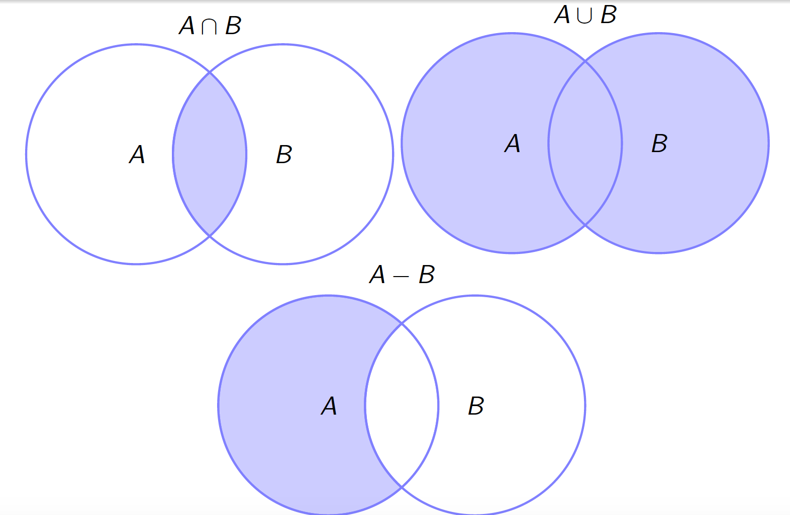
\(A\cap B\): the intersection of \(A\) and \(B\) is the subset of \(S\) that contains all the elements that are in both \(A\) and \(B\);
\(A\cup B\): the union of \(A\) and \(B\) is the subset of \(S\) that contains all the elements that are either in \(A\), in \(B\), or in both;
\(A-B\): the difference of \(A\) and \(B\) is the subset of \(A\) that contains all the elements of \(A\) that are not in \(B\);
\(\overline{A}\) (or \(A'\)): the complement of \(A\) is the subset of \(S\) that contains all the elements of \(S\) that are not in \(A\), i.e. \(\overline{A}=S-A\).
3.5 Venn Diagrams
3.6 Properties of Operations with Events
Let \(A, B\) and \(C\) be events of \(S\). Then, the following properties hold true:
Associativity: \[(A\cup B)\cup C=A\cup(B\cup C),\quad\text{and}\quad (A\cap B)\cap C=A\cap(B\cap C)\]
Comutatitvity: \[A\cup B=B\cup A\quad\text{and}\quad A\cap B=B\cap A\]
Distributivity: \[A\cup(B\cap C)=(A\cup B)\cap (A\cup C)\quad\text{and}\quad A\cap(B\cup C)=(A\cap B)\cup (A\cap C)\]
De Morgan’s Laws: \[\overline{A\cup B}=\overline{A}\cap\overline{B}\quad\text{and}\quad\quad \overline{A\cap B}=\overline{A}\cup\overline{B}\]
Mutually Exclusive Events: Two events having no elements in common are said to be mutually exclusive (or Disjoint or Incompatible). In other words, the events \(A\) and \(B\), with \(A,B\subset S\), are disjoint if \[A\cap B=\emptyset.\]
Prove the following properties:
Let \(A\) and \(B\) be two events of \(S\), the sample space.
\(A\cup A=A\cap A=A\);
\(A\subset B\Rightarrow A\cap B=A\) and \(A\cup B=B\);
\(A\cap S=A\cup\emptyset=A;\)
\(\overline{\overline{A}}=A;\)
\(A\cap\overline{A}=\emptyset\) (\(A\) and \(\overline{A}\) are mutually exclusive events);
\(A\cup\overline{A}=S.\)
\(A-B=A\setminus B=A\cap\overline{B}\)
4 Kolmogorov’s postulates and properties
4.1 Probability Space
A probability space is a triplet \((S,{\cal F}, P)\), where \(S\) is the sample space, \({\cal F}\) is a \(\sigma-\)algebra and \(P\) is a probability measure.
Roughly speaking, \({\cal F}\) is a collection of all events contained in \(S\), i.e., \({\cal F}=\{A_1,A_2,A_3,\cdots\}\).
Definition: A \(\sigma-\)algebra \(\cal F\) is a set of events that satisfies the following properties:
\(\cal F\) contain the sample space \((S\in {\cal F})\);
If \(A\in{\cal F}\), then \(\overline{A}\in{\cal F}\);
If \(A_1, A_2, A_3, \cdots\), then \(\bigcup_{i=1}^{+\infty}A_i\in{\cal F}\)
Example 4.1 Sample Space: \(S=\{H,T\}\);
\(\sigma-\)algebra: \({\cal F}=\{S,\emptyset,\{H\},\{T\}\}\)
With the probability measure, we assigna probability to each event in \(\cal F\)
4.2 Properties of \(P\)
A probability measure is a function with domain \({\cal F}\) that satisfies the Kolmogorov Axioms:
\(P(S)=1\)
\(P(A)\geq 0\), for all \(A\in{\cal F}\)
If \(A_1, A_2, A_3, \cdots\) are mutually exclusive events, then \[P(\bigcup_{i=1}^{+\infty}A_i)=\sum_{i=1}^{+\infty}P(A_i).\]
Theorem: Let \(A\) and \(B\) be two events of \(S\). The following properties follow from the Kolmogorov Axioms.
\(P(\overline{A})=1-P(A)\) and \(P(\emptyset)=0\);
\(A\subset B\Rightarrow P(A)\leq P(B)\);
\(P(A)\leq 1\);
\(P(B- A)=P(B)-P(A\cap B)\);
\(P(A\cup B)=P(A)+P(B)-P(A\cap B)\).
Prove the previous Theorem!
- \(P(\overline{A})=1-P(A)\);
Proof: We know that \(A\cup \overline{A}=S\). Then, \[\begin{aligned} P(S)&=P(A\cup \overline{A})=\underbrace{P(A)+P(\overline{A})}_{A\text{ and }\overline{A}\text{ are disjoint}}\\ \Leftrightarrow 1&= P(A)+P(\overline{A}) \end{aligned}\]
- \(P(\emptyset)=0\);
Proof: Notice that \(\overline{S}=\emptyset\). Then, from the previous property, we get that \[P(\emptyset)=P(\overline{S})=1-P(S)=1-1=0.\]
- \(A\subset B\Rightarrow P(A)\leq P(B)\);
Proof: If \(A\subset B\), then \(B=A\cup(B-A)\). Additionally \(A\cap (B-A)=\emptyset\) (Check these two statements!)
Therefore, \[\begin{aligned} P(B)=P(A\cup (B-A))=\underbrace{P(A)+ P((B-A))}_{A\text{ and }(B-A)\text{ are disjoint}}. \end{aligned}\]
Since \(P((B-A))\geq 0\), then \(P(B)\geq P(A)\).
- \(P(A)\leq 1\);
Proof: Since \(A\subset S\), then \(P(A)\leq P(S)=1\).
- \(P(B- A)=P(B)-P(A\cap B)\);
Proof: We stat by noticing that \(B=(B-A)\cup(A\cap B)\). Additionally, \((B-A)\cap(A\cap B)=\emptyset\). (Check these two statements!). \[\begin{aligned} P(B)=P((B-A)\cup(A\cap B))=\underbrace{P(B-A)+P(A\cap B)}_{A\cap B\text{ and }(B-A)\text{ are disjoint}} \end{aligned}\]
- \(P(A\cup B)=P(A)+P(B)-P(A\cap B)\).
Proof: We start by noticing that \(A\cup B=(A-B)\cup(A\cap B)\cup (B-A)\). Then, \[\begin{aligned} P(A\cup B)&=P(A-B)+P(A\cap B)+P(B-A)\\ &=P(A)+P(B)-P(A\cap B), \end{aligned}\] the second equality following from the previous property.
5 Interpretations of the concept of probability
5.1 Laplace’s definition of probability
Let \(S\) be a sample space such that
\(S\) is composed of \(n\) elements \((\# S=n)\)
all outcomes are distinct and equally likely.
Let \(A\) be an event of \(S\): \[P(A)=\frac{\# A}{\# S}.\]
Example 5.1 \(S=]0,+\infty[\) and \(\# S=+\infty\). Then, it is not possible to use the Laplace’s definition of probability.
Example 5.2 \(S=\{(R,G)\,: R,G=1,2,3,4,5,6\}\) and \(A=\) “The sum of dots in both dice is greater than \(9\).” \(A=\{(4,6),(5,5),(6,4),(5,6),(6,5),(6,6)\}\). \[P(A)=\frac{\# A}{\# S}=\frac{6}{36}=\frac{1}{6}\]
5.2 Relative frequency definition of probability
Relative frequency of an event \(A\): Repeat an experiment \(N\) times and assume that the event \(A\) occurs \(n_A\) times throughout these \(N\) repetitions. Then, we say that the relative frequency of \(A\) is \[f_N(A)=\frac{n_A}{N}.\]
Remark: \(f_N\) satisfies the following properties:
\(0\leq f_N(A)\leq 1\), for all \(A\in S\)
\(f_N(S)=1\)
\(f_N(A\cup B)=f_N(A)+f_N(B)\), if \(A\cap B=\emptyset\)
Frequencist interpretation of probability: The frequncist probability of the event \(A\) is given by: \[\lim_{N\to +\infty}f_N(A)=P(A).\] This is also known as Law of Large Numbers.
Example 5.3 A regular coin is tossed 300 times. The number of times that a tail occurred throughout these 300 repetitions was counted.
Relative frequency of occurrence of a tail.
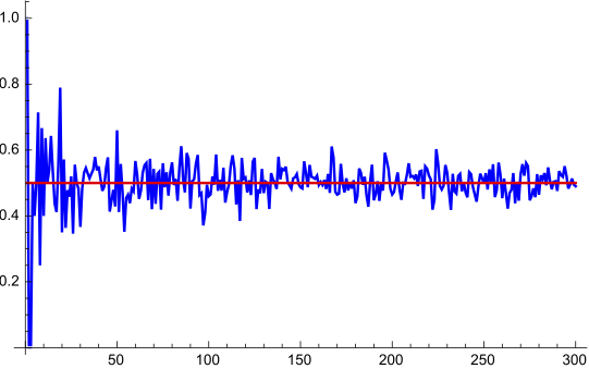
It is clear that: \[P("\text{A tail is obtained}")=\lim_{N\to+\infty}=\frac{1}{2}\]
\(N\)
5.3 Subjective interpretation of probability
The subjective definition of probability deals with the problem of calculating probabilities when the experiment is not symmetric and cannot be successively repeated.
Let \(A\) be an event of \(S\). The subjective probability of \(A\) is a number in \([0,1]\) that represents the degree of confidence that a person assigns to the occurrence of \(A\).
Example 5.4 The probability that each one assigns to the event \(B=\)"The price is greater then \(170\$\)" depends on their knowledge about the stock market.
For me \(P(B)=0.5\) but for a market analyst \(P(B)=?\).
6 Conditional Probability
How can we assign a probability to an event when we have partial information about the outcome of the random experiment?
Example 6.1 \(S=\{(R,G)\,: R,G=1,2,3,4,5,6\}\) and \(A=\) “The sum of dots in both dice is greater than \(9\).” \(A=\{(4,6),(5,5),(6,4),(5,6),(6,5),(6,6)\}\). \[P(A)=\frac{\# A}{\# S}=\frac{6}{36}=\frac{1}{6}\] Consider now the event \(\tilde A=\)" The sum of dots in both dice is greater than \(9\) given that at least one die has an upper face with 5 dots". Then, \[P(\tilde A)=3/11.\] Is this correct?
Conditional probability: Let \(A\) and \(B\) be two events in a sample space \(S\) such that \(P(B)\neq 0\). Then, the conditional probability of \(A\) given that \(B\) has occurred is \[P(A\vert B)=\frac{P(A\cap B)}{P(B)}.\] Remark:
The logic behind this equation is that if the possible outcomes for A and B are restricted to those in which B occurs, this set serves as the new sample space;
\(P(\cdot\vert B)\) is a new probability measure.
The probability measure \(P(\cdot\vert B)\) satisfies the Kolmogorov Axioms:
\(P(S\vert B)=1\)
\(0\leq P(A\vert B)\leq 1\), for all \(A\in{\cal F}\)
If \(A_1, A_2, A_3, \cdots\) are mutually exclusive events, then \[P(\bigcup_{i=1}^{+\infty}A_i)=\sum_{i=1}^{+\infty}P(A_i).\]
Example 6.2 \(S=\{(R,G)\,: R,G=1,2,3,4,5,6\}\), \(A=\) “The sum of dots in both dice is greater than \(9\)”, \(B=\) “At least one die has an upper face with 5 dots” and \(\tilde A=\)" The sum of dots in both dice is greater than \(9\) given that at least one die has an upper face with 5 dots".Then, \[P(\tilde A)=P(A\vert B)=\frac{P(A\cap B)}{P(B)}=\frac{3}{11}.\]
6.1 Multiplication rule
Let \(A\) and \(B\) be two events in a sample space \(S\) such that \(P(B)\neq 0\). Then, the multiplication rule \[P(A\cap B)=P(A\vert B)\times P(B).\] In the same way, if \(P(A)\neq 0\), then \[P(A\cap B)=P(B\vert A)\times P(A).\]
Example 6.3 We draw successively at random and without replacement 2 cards from a full deck of cards. What is the probability that we draw in order 1 Heart (H) and 1 Diamond (D)? \[\begin{aligned} P(``\text{draw 1 Heart (H) and 1 Diamond (D)}'')=\\ =P(H)\times P(D|H)=\frac{13}{52}\times\frac{13}{51}\end{aligned}\]
The multiplication rule can be generalized for \(3,4,5,\cdots\) events.
Theorem: Let \(A\), \(B\) and \(C\) be three events in a sample space \(S\) such that \(P(B\cap C)\neq 0\). Then, the multiplication rule is \[P(A\cap B\cap C)=P(C)\times P(B\vert C)\times P(A\vert B\cap C).\] Proof: By definition \[P(A\vert B\cap C)=\frac{P(A\cap B\cap C)}{P(B\cap C)}\text{ and }P(C)\times P(B\vert C)=P(B\cap C).\] Therefore, \[P(C)\times P(B\vert C)\times P(A\vert B\cap C)= P(A\cap B\cap C).\]
Example 6.4 We draw successively at random and without replacement 3 cards from a full deck of cards. What is the probability that we draw in order 1 Heart (H), 1 Heart (H) and 1 Diamond (D)?
\[ \begin{aligned} P(``\text{draw 1 Heart (H), 1 Heart and 1 Diamond (D)}'')=\\ =P(H)\times P(H|H)\times P(D\vert H\cap H)=\frac{13}{52}\times\frac{12}{51}\times\frac{13}{50}. \end{aligned} \] Suppose know that we draw 4 cards. What is the probability that we draw in order 1 Heart (H), 1 Heart (H), 1 Diamond (D) and 1 Club (C).
\[ \begin{aligned} &P(``\text{draw 1 Heart (H), 1 Heart, 1 Diamond (D) \,and \,1 Club (C)}'')=\\ &P(H)P(H|H)P(D\vert H\cap H)P(C\vert H\cap H\cap D)=\frac{13}{52}\times\frac{12}{51}\times\frac{13}{50}\times \frac{13}{49}. \end{aligned} \] ## Partition
Partition: Let \(A_1, A_2, \cdots, A_n\) be \(n\) events of \(S\). We say that \(A_1, A_2, \cdots, A_n\) is a partition to \(S\) whenever the following conditions are satisfied:
the events \(A_1, A_2, \cdots, A_n\) are pairwise disjoint: \[A_i\cap A_j=\emptyset,\quad\forall i\neq j\in\{1,2,\cdots n\};\]
the of all events is the sample space: \[\bigcup_{i=1}^n A_i= S.\]
Remark:
If \(B\subset S\), then \[B=\bigcup_{i=1}^{n}(A_i\cap B);\]
If \(A\subset S\), then \(\{A,\overline{A}\}\) is a partition of \(S\).
6.2 Total probability theorem
Total probability theorem: Let \(B\) be an event of \(S\) and \(A_1, A_2, \cdots, A_n\) a partition of \(S\) such that \(P(A_j)>0\), for all \(j=1,2,\cdots,n\). Then,
\[ \begin{aligned} P(B)&=\sum_{i=1}^n P(B\vert A_i)\times P(A_i)\\ &=\sum_{i=1}^n P(B\cap A_i) \end{aligned} \] Proof: The result comes from the previous remark and the multiplication rule.
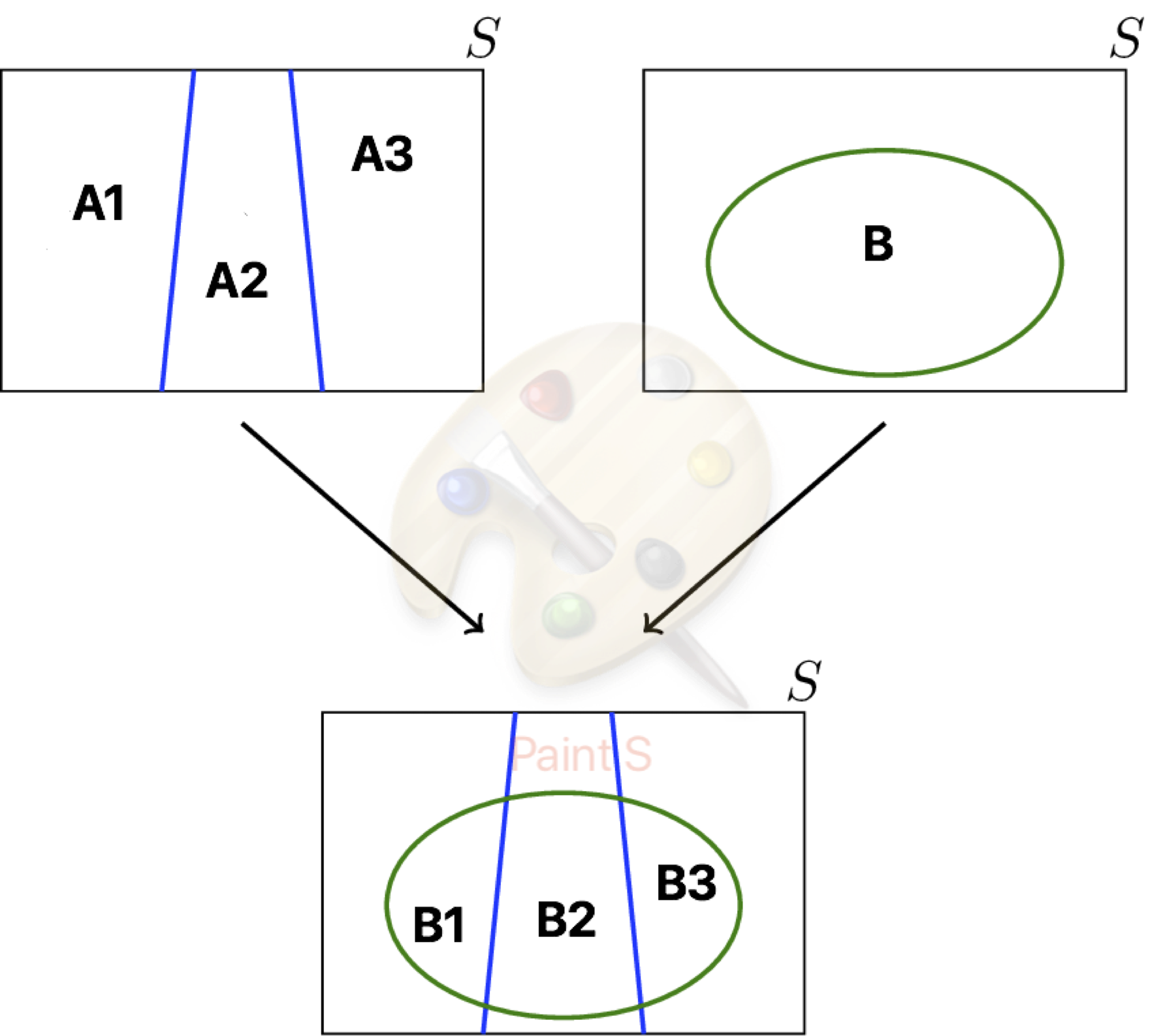
where the events \(B_i\), with \(i=1,2,3\), are such that \[B_i=B\cap A_i.\]
6.3 Bayes’ theorem
Bayes’ theorem: Let \(B\) be an event of \(S\) and \(A_1, A_2, \cdots, A_n\) a partition of \(S\). Additionally, assume that \(P(B)>0\) and \(P(A_j)>0\), for all \(j=1,2,\cdots,n\). Then, \[\begin{aligned} P(A_j\vert B)&=\frac{P(A_j)\times P(B\vert A_j)}{P(B)}\\ &=\frac{P(A_j)\times P(B\vert A_j)}{\sum_{i=1}^n P(B\cap A_i)}\\ &=\frac{P(A_j)\times P(B\vert A_j)}{\sum_{i=1}^n P(A_i)\times P(B\vert A_i)} \end{aligned} \]
Proof: By definition, \[P(A_j\vert B)=\frac{P(A_j\cap B)}{P(B)}.\]
Use the multiplication rule to rewrite the numerator and the total probability law to rewrite the denominator.
6.4 Examples
Example 6.5 If we randomly pick a blue ball, what is the probability of being from the first box?
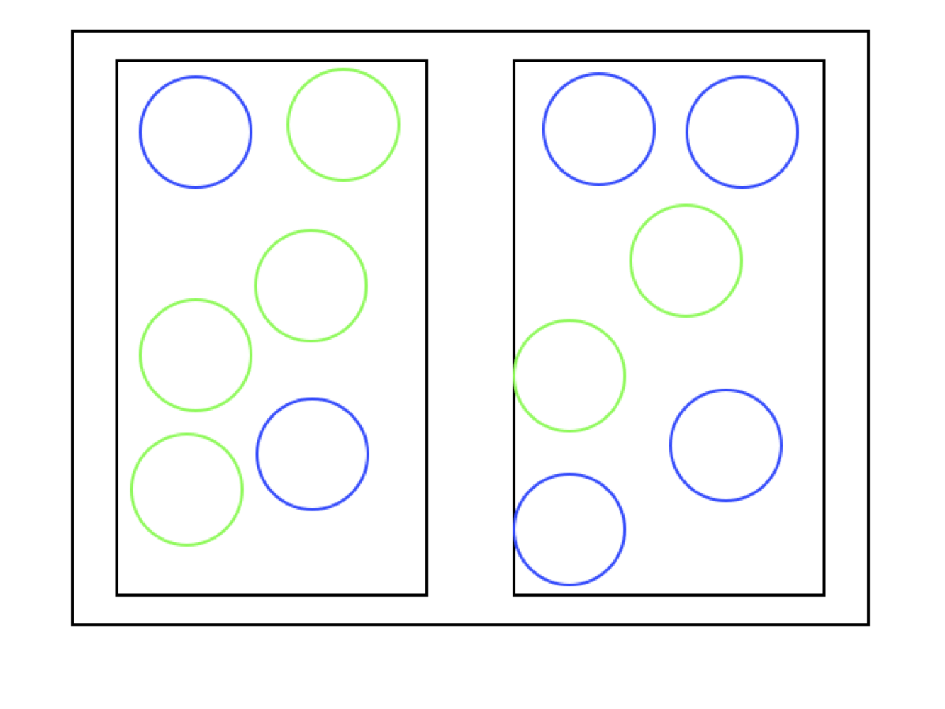
image
\[ P(\mbox{Choose box 1})=\frac{1}{2} \]
Let’s start from the beginning:
\(A=``\)Select a blue ball\("\) \(B_i=\)“Choose box" \(i\), \(i=1,2\).
\(P(A\vert B_1)=\frac{1}{3},\quad P(A\vert B_2)=\frac{2}{3}\)
\(P(A)=?\)
Example 6.6 If we draw randomly a blue ball, what is the probability of being in the first box?
image
\[ \begin{aligned} P(B_i)=\frac{1}{2},\quad P(A\vert B_1)=\frac{1}{3}\\ P(A\vert B_2)=\frac{2}{3} \end{aligned} \]
From the total probability theorem: \[ \begin{aligned} P(A)&=P(A\cap B_1)+P(A\cap B_2)\\ &=P(A\vert B_1)P(B_1)\\ &+P(A\vert B_2)P(B_2)=\frac{1}{2} \end{aligned} \] Then,
\[ \begin{aligned} P(B_1\vert A)=&\frac{P(A\vert B_1)P(B_1)}{P(A)}\\ =&\frac{1/6}{1/2}=\frac{1}{3} \end{aligned} \]
Example 6.7 Suppose that a firm has to face three different scenarios: the demand increases, decreases or maintains equal. Additionally, the price can also increase, decrease or maintain equal.
| Price/Demand | \(\nearrow\) | \(\searrow\) | \(=\) | Total |
|---|---|---|---|---|
| \(\nearrow\) | \(0.1\) | \(0.3\) | \(0.15\) | \(0.55\) |
| \(\searrow\) | \(0.1\) | \(0.05\) | \(0.05\) | \(0.2\) |
| \(=\) | \(0.05\) | \(0.1\) | \(0.1\) | \(0.25\) |
| Total | \(0.25\) | \(0.45\) | \(0.30\) | \(1\) |
Compute the probability that the price increases (PI) and probability that the demand increases (PI). \[P(PI)=0.55\quad\text{and}\quad P(DI)=0.25\]
Example 6.8 Compute the probability that the price increases (PI) given that the demand increases (DI).
\[ P(PI~\vert~ DI)=\frac{P(PI~\cap~ DI)}{P(DI)}=\frac{0.1}{0.25}=\frac{2}{5}. \]
Compute the probability that the demand increase (DI) given that the price increases (PI). \[ \begin{aligned} P(DI~\vert~ PI)=&\frac{P(PI~\vert~ DI)P(DI)}{P(PI)}\\ =&\frac{P(PI~\cap~ DI)}{P(PI)}=\frac{2}{11} \end{aligned} \]
7 Independent Events
Independence: Two events \(A\) and \(B\) of \(S\) are independent when \(P(A\cap B) = P(A)\times P(B)\).
Remark: This definition is equivalent to:
\(P(A\vert B)=P(A)\), if \(P(B)>0\).
\(P(B\vert A)=P(B)\), if \(P(A)>0\).
Independence of more than two events: The events \(A_1, A_2, \cdots , A_k\) of are independent when the probability of the intersections of any \(2, 3, \cdots, k\) of these events equals the product of their respective probabilities.
Example: When \(k=3\), \(A_1, A_2\) and \(A_3\) are independent if \[ \begin{aligned} P(A_i\cap A_j)=P(A_i)\times P(A_j),\quad \text{for all }i\neq j\in{i,2,3}\\ P(A_1\cap A_2\cap A_3)=P(A_1)\times P(A_2)\times P(A_3) \end{aligned} \]
Properties: Let \(A\) and \(B\) be independent events of \(S\). Then the following assertions hold true:
\(A\) and \(\overline{B}\) are independent events;
If \(A\) and \(B\) are disjoint and \(P(A)=0\) or \(P(B)=0\), then \(A\) and \(B\) are independent events; and
If \(A\) and \(B\) are disjoint, \(P(A)>0\) and \(P(B)>0\), then \(A\) and \(B\) are not independent events.
Proof of 1): Notice that \[\begin{aligned} P(A\cap \overline{B})&=P(A-B)=P(A)-P(A\cap B)\\ &=P(A)-P(A)\times P(B)=P(A)\left(1-P(B)\right)\\ &=P(A)\times P(\overline{B}). \end{aligned} \]
Example 7.1 Suppose that a firm has to face three different scenarios: the demand increases, decreases or maintains equal. Additionally, the price can also increase, decrease or maintain equal.
| Price/Demand | \(\nearrow\) | \(\searrow\) | \(=\) | Total |
|---|---|---|---|---|
| \(\nearrow\) | \(0.1\) | \(0.3\) | \(0.15\) | \(0.55\) |
| \(\searrow\) | \(0.1\) | \(0.05\) | \(0.05\) | \(0.2\) |
| \(=\) | \(0.05\) | \(0.1\) | \(0.1\) | \(0.25\) |
| Total | \(0.25\) | \(0.45\) | \(0.30\) | \(1\) |
Are the events \(PI\) and \(DI\) independent?
No, because \(0.1=P(PI\cap DI)\neq P(DI)\times P(PI)=0.1375\).