3. Expected Values
1 Motivation
To describe an experiment (a random experiment), we oftenly use measures that allow us to summarize the available data. The “mean" is one of that measures, since it helps us to localize the center of the distribution. For example:
Example 1.1 Students that enroll the postgraduate in Finance have to complete 4 curricular units 2 of them with 10 ECTS and the remaining 2 with 5 ECTS. João has completed the postgraduate in Finance with the following marks:
15 - course with 10 ECTS
13 - course with 10 ECTS
16 - course with 5 ECTS
14 - course with 5 ECTS
The average final grade of João was \(14\), since \[\frac{15\times 10+13\times 10+16\times 5+14\times 5}{30}=14.(3)\]
2 The Expected Value of A Random Variable
2.1 Discrete Random Variables
Let \(X\) be a a discrete random variable and let \(D_{X}\) be the set of discontinuity points of the cumulative distribution function \(X.\) For generality, let us assume that the number of elements of \(D_{X}\) is countably infinite, that this \(D_{X}=\left \{ x_{1},x_{2},...\right \} .\)
The probability function of \(X\) is given by \[f_{X}\left( x\right) =\left \{ \begin{array}{cc} P\left( X=x\right) & ,x\in D_{X} \\ 0 & ,x\notin D_{X}% \end{array}% \right.\]
Expected Value of a discrete random variable: The expected value of a random variable, denoted as \(E\left( X\right)\) or \(\mu _{X}\), also known as its population mean, is the weighted average of its possible values, the weights being the probabilities attached to the values \[\mu _{X}=E\left( X\right) =\sum_{x\in D_{X}}x\times f_{X}\left( x\right) =\sum \limits_{i=1}^{\infty }x_{i}\times f_{X}\left( x_{i}\right) .\] provided that \(\sum_{x\in D_{X}}\left \vert x\right \vert \times f_{X}\left( x\right) =\sum \nolimits_{i=1}^{\infty }\left \vert x_{i}\right \vert \times f_{X}\left( x_{i}\right) <+\infty .\)
Example 2.1 Let \(X\) be a discrete random variable such that \[X=\begin{cases} 1, & \text{if there is a success}\\ 0, &\text{otherwise} \end{cases}\text{ and } P(X=x)=\begin{cases} p,& \text{if }x=1\\ 1-p,& \text{if }x=0 \end{cases}.\] The expected value of \(X\) is given by \[E(X)=p\times 1 + (1-p)\times 0=p\]
Remarks:
If the number of elements of \(D_{x}\) is finite that this \(% D_{X}=\left \{ x_{1},x_{2},...,x_{k}\right \}\) where \(k\) is a finite integer, then \(\sum_{x\in D_{X}}\left \vert x\right \vert \times f_{X}\left( x\right) =\sum \nolimits_{i=1}^{k}\left \vert x_{i}\right \vert \times f_{X}\left( x_{i}\right)\) and the condition \(\sum \nolimits_{i=1}^{k}\left \vert x_{i}\right \vert \times f_{X}\left( x_{i}\right) <+\infty\) is always satisfied.
Note that \(\mu _{X}\) can take values that are not in \(D_{X}.\)
Example: Let \(X\) be the random variable with the probability function \[P(X=2^n)=2^{-n}, \quad\text{for all $n\in\mathbb{N}$}.\] This means that \(P(X=x)=0\) for all \(x\notin\{2^n\,:n\in\mathbb{N}\}\). One can notice that the probability function satisfies the conditions:
\(P(X=x)\geq 0\) for all \(x\in\mathbb{R}\);
\(\sum_x P(X=x)=\sum_{n=1}^\infty 2^{-n}=\frac{1/2}{1-1/2}\)
Additionally, one may easily notice that, the distribution does not have expected value: \[E(X)=\sum_{n=1}^\infty2^n\times 2^{-n}=\infty\]
2.2 Continuous Random Variables
Expected values (or mean or expectation) of a continuous random variable: If \(X\) is a continuous random variable and \(f_{X}(x)\) is its probability density function at \(x,\) the expected value of \(X\) is \[\mu _{X}=E(X)=\int_{-\infty }^{+\infty }xf_{X}(x)dx\] provided that \(\int_{-\infty }^{+\infty }\left \vert x\right \vert f_{X}(x)dx<\infty .\)
Remark: Thus, the mean can be thought of as the centre of the distribution and, as such, it describes its location. Consequently, the mean is considered as a measure of location.
Example 2.2 Let \(X\) be a random variable with probability density function given by \[f_X(x)=\begin{cases} \frac{1}{b-a},&a<x<b\\ 0,& \text{otherwise} \end{cases}.\]
Then, the expected value of \(X\) is \(E(X)=\int_{-\infty}^{+\infty}xf_X(x)dx=\int_{a}^{b}\frac{x}{b-a}dx=\frac{b+a}{2}\)
Expected value of a function of a discrete random variable: If \(X\) is a discrete random variable and \(f_{X}(x)\) is the value of its probability function at \(x,\) the expected value of \(\ g\left( X\right)\) is \[E\left[ g\left( X\right) \right] =\sum_{x\in D_{X}}g\left( x\right) \times f_{X}\left( x\right) =\sum \limits_{i=1}^{\infty }g\left( x_{i}\right) \times f_{X}\left( x_{i}\right) .\] provided that \(\sum_{x\in D_{X}}\left \vert g\left( x\right) \right \vert \times f_{X}\left( x\right) =\sum \nolimits_{i=1}^{\infty }\left \vert g\left( x_{i}\right) \right \vert \times f_{X}\left( x_{i}\right) <+\infty .\)
Expected value of a function of a continuous random variable: If \(X\) is a continuous random variable and \(f_{X}(x)\) is its probability density function at \(x,\) the expected value of \(g\left( X\right)\) is \[E\left( g\left( X\right) \right) =\int_{-\infty }^{+\infty }g(x)f(x)dx.\] provided that \(\int_{-\infty }^{+\infty }\left \vert g\left( x\right) \right \vert f_{X}(x)dx<\infty .\)
Remark:
- The existence of \(E\left( X\right)\) does not imply the existence of \(E\left( g\left( X\right) \right)\) and vice versa.
3 The Mean of A Function of A Random Variable
- \(E\left( g\left( X\right) \right)\) can be calculated using the above definition or finding the distribution of \(Y=g\left( X\right)\) and computing directly \(E\left( Y\right) .\)
Example: Let \(X\) be a discrete random variable with probability function given by \(f_{X}\left( x\right) =1/3,\) \(x=-1,\) \(0,\) \(1\) and \(Y=g(X)=X^{2}.\) We can compute \(E(X^{2})\) if the following two ways:
By using the definition of expected value of a function of a random variable \[\begin{aligned} E\left( X^{2}\right) &=\left( -1\right) ^{2}f_{X}\left( -1\right) +\left( 0\right) ^{2}f_{X}\left( 0\right) +\left( 1\right) ^{2}f_{X}\left( 1\right) \\ &=1\times 1/3+0\times 1/3+1\times 1/3=2/3.\end{aligned}\]
Finding the distribution of \(Y\) and afterwards computing the expected value of \(Y\). \[\begin{aligned} &f_{Y}\left( 0\right) =P(Y=0)=P(X=0)=1/3\\ &f_{Y}\left(1\right) =P(Y=1)=P(X=-1)+P(X=1)=1/3+1/3=2/3. \end{aligned}\]
Therefore, \[f_Y(y)=\begin{cases} 1/3,&y=0\\ 2/3,&y=1\\ 0,&\text{otherwise} \end{cases}.\] Thus, \(% E(X^{2})=E(Y)=0\times f_{Y}\left( 0\right) +1\times f_{Y}\left( 1\right) =0\times 1/3+2\times 1/3=2/3.\)
Example: Let \(X\) be a random variable such that \[f_X(x)=\begin{cases} \frac{1}{b-a},&a<x<b\\ 0,&\text{otherwise}\end{cases}.\] Then, the expected value of \(Y=2X\) is
\[E(2X)=\int_{-\infty}^{+\infty}2xf_{X}(x)dx=\int_{a}^{b}2\frac{x}{b-a}dx=2\int_{a}^{b}\frac{x}{b-a}dx=b+a.\]
A different approach to calculate \(E(Y)\) is to derive the distribution of \(Y\) and afterwards to compute \(E(Y)\).
Indeed, \[F_Y(y)=P(Y\leq y)=P(2X\leq y)=P(X\leq y/2)=F_X(y/2).\]
The density function can be obtaining differentiating the cdf \(F_Y\): \[\begin{aligned} f_Y(y)&=F'_Y(y)=(F_X(y/2))'=\frac{1}{2}F'_X(y/2)=\frac{1}{2}f_X(y/2)\\ &=\begin{cases} \frac{1}{2(b-a)},&2a<y<2b\\ 0,& \text{otherwise} \end{cases} \end{aligned}\]
Therefore,
\[E(Y)=\int_{-\infty}^{+\infty}yf_Y(y)dy=\int_{2a}^{2b}\frac{y}{2(b-a)}dy=b+a\]
4 Properties of The Expected Value
The expected values satisfy the following properties:
\(E(a+bX)=a+bE\left( X\right) ,\) where \(a\) and \(b\) are constants\(.\)
\(E(X-\mu _{X})=E\left( X\right) -\mu _{X}=0.\)
If \(a\) is a constant, \(E\left( a\right) =a.\)
If \(b\) is a constant, \(E\left( b\times g\left( X\right) \right) =bE\left( g\left( X\right) \right) .\)
Given \(n\) functions \(u_{i}\left( X\right)\) \(i=1,...,n\) and \(,\) \(E% \left[ \sum_{i=1}^{n}u_{i}\left( X\right) \right] =\sum_{i=1}^{n}E\left[ u_{i}\left( X\right) \right] .\)
5 Higher Order Raw Moments and Centered Moments
Moments of a discrete random variable: The \(r^{th}\) moment of a discrete random variable (or its distribution), denoted as \(\mu _{r}^{\prime }\), is the expected value of \(X^{r}\) \[\mu _{r}^{\prime }=E\left( X^{r}\right) =\sum_{x\in D_{X}}x^{r}\times f_{X}\left( x\right) =\sum \limits_{i=1}^{\infty }x_{i}^{r}\times f_{X}\left( x_{i}\right) ,\text{ for }r=1,2,...\] provided that \(\sum_{x\in D_{X}}\left \vert x\right \vert ^{r}\times f_{X}\left( x\right) =\sum \nolimits_{i=1}^{\infty }\left \vert x_{i}\right \vert ^{r}\times f_{X}\left( x_{i}\right) <+\infty .\)
Moments of a continuous random variable: The \(r^{th}\) moment of a continuous random variable (or its distribution), denoted as \(\mu _{r}^{\prime }\), is the expected value of \(X^{r}:\) \[\mu _{r}^{\prime }=E(X^{r})=\int_{-\infty }^{+\infty }x^{r}f_{X}(x)dx\] provided that \(\int_{-\infty }^{+\infty }\left \vert x\right \vert ^{r}f_{X}(x)dx<\infty .\)
\(r^{th}\) central moment of the random variable or \(r^{th}\) moment of a random variable about its mean
Central moments of a discrete random variable: The \(r^{th}\) central moment of a discrete random variable (or its distribution), denoted as \(\mu _{r}\), is the expected value of \(\left( X-\mu _{X}\right) ^{r}\) \[\mu _{r}=E\left[ \left( X-\mu _{X}\right) ^{r}\right] =\sum_{x\in D_{X}}\left( x-\mu _{X}\right) ^{r}\times f_{X}\left( x\right) =\sum \limits_{i=1}^{\infty }\left( x_{i}-\mu _{X}\right) ^{r}\times f_{X}\left( x_{i}\right) ,\text{ for }r=1,2,...\] provided that \(\sum_{x\in D_{X}}\left \vert x-\mu _{X}\right \vert ^{r}\times f_{X}\left( x\right) =\sum \nolimits_{i=1}^{\infty }\left \vert x_{i}-\mu _{X}\right \vert ^{r}\times f_{X}\left( x_{i}\right) <+\infty .\)
Central moments of a continuous random variable: The \(r^{th}\) central moment of a continuous random variable (or its distribution), denoted as \(% \mu _{r}\), is the expected value of \(\left( X-\mu _{X}\right) ^{r}:\) \[\mu _{r}=E\left[ \left( X-\mu _{X}\right) ^{r}\right] =\int_{-\infty }^{+\infty }\left( x-\mu _{X}\right) ^{r}f_{X}(x)dx\] provided that \(\int_{-\infty }^{+\infty }\left \vert x-\mu _{X}\right \vert ^{r}f_{X}(x)dx<\infty .\)
Example 5.1 Let \(X\) be a random variable such that \(f_X(x)=\frac{1}{b-a}\) if \(a<x<b\), and \(f_X(x)=0\) if \(x\notin(a,b)\).
The \(2^{\text{nd}}\) moment is \[\begin{aligned} \int_{-\infty}^{+\infty}x^2f_X(x)dx=\int_{a}^{b}\frac{x^2}{b-a}dx=\frac{1}{3}(a^2+ab+b^2).\end{aligned}\]
The \(2^{\text{nd}}\) central moment is \[\begin{aligned} \int_{-\infty}^{+\infty}(x-\mu_X)^2f_X(x)dx=\int_a^{b}\frac{(x-\mu_X)^2}{b-a}dx=\frac{(b-a)^2}{12}.\end{aligned}\]
\(\mu _{1}\) is of no interest because is it zero when it exists.
\(\mu _{2}\) is an important measure and is called variance.
\(\mu _{3}\) and \(\mu _{4}\) are also important.
5.1 The Variance of a Random Variable
Variance: the second central moment about the mean of a random variable (\(\mu _{2}\)), also called variance, is an indicator of the dispersion of the values of \(X\) about the mean.
The variance of a discrete random variable: \[Var\left( X\right) =\sigma _{X}^{2}=\mu _{2}=E\left[ \left( X-\mu _{X}\right) ^{2}\right] =\sum_{x\in D_{X}}\left( x-\mu _{X}\right) ^{2}\times f_{X}\left( x\right),\] provided that \(Var\left( X\right) <+\infty .\)
The variance of a continuous random variable: \[Var\left( X\right) =\sigma _{X}^{2}=\mu _{2}=E\left[ \left( X-\mu _{X}\right) ^{2}\right] =\int_{-\infty }^{+\infty }\left( x-\mu _{X}\right) ^{2}f_{X}(x)dx,\text{ }\] provided that \(Var\left( X\right) <+\infty .\)
Remark: We can show that if \(\mu _{2}^{\prime }=E\left( X^{2}\right)\) exists, then both \(\mu _{X}\) and \(\sigma _{X}^{2}\) exist.
Properties of the Variance:
\(Var\left( X\right) \geq 0.\)
\(\sigma _{X}^{2}=Var\left( X\right) =E\left( X^{2}\right) -\mu _{X}^{2}.\)
If \(c\) is a constant, \(Var\left( c\right) =0.\)
If \(a\) and \(b\) are constants, \(Var\left( a+bX\right) =b^{2}Var\left( X\right) .\)
Example 5.2 Let \(X\) be a discrete random variable such that \[X=\begin{cases} 1, & \text{if there is a success}\\ 0, &\text{otherwise} \end{cases}\text{ and } P(X=x)=\begin{cases} p,& \text{if }x=1\\ 1-p,& \text{if }x=0 \end{cases}.\] The expected value of \(X\) is given by \[\begin{aligned} E(X)&=p\times 1 + (1-p)\times 0=p\\ E(X^2)&=p\times 1^2 + (1-p)\times 0^2=p\\ Var(X)&=E(X^2)-(E(X))^2=p(1-p) \end{aligned}\]
Example 5.3 Let \(X\) be a continuous random variable such that \[f_X(x)=\begin{cases} 2x,&0<x<1\\ 0,& \text{otherwise} \end{cases}.\] Then, \[E(X)=\int_{-\infty }^{+\infty}xf_X(x)dx=2/3\] and \[E(X^2)=\int_{-\infty }^{+\infty}x^2f_X(x)dx=1/2.\] Therefore, \[Var(X)=E(X^2)-(E(X))^2=\frac{1}{18}\]
Standard deviation: The variance is not measured in the scale of the random variable as it is computed using the square function, in order to obtain a measure of dispersion about the mean which is measure in the same scale of the random variable we need to compute the standard deviation. The Standard deviation is given by: \[\sigma _{X}=\sqrt{Var\left( X\right) }.\]
5.2 Coefficient of Variation, Skewness and Kurtosis
Other Population Distribution Summary Statistics are:
Coefficient of variation: If we are interested in a measure of dispersion which is independent of the scale of the random variable we should use the coefficient of variation. The coefficient of variation is given by \[CV\left( X\right) =\frac{\sigma _{X}}{\mu _{X}}.\]
Example 5.4 Let \(X\) be a discrete random variable such that \[X=\begin{cases} 1, & \text{if there is a success}\\ 0, &\text{otherwise} \end{cases}\text{ and } P(X=x)=\begin{cases} p,& \text{if }x=1\\ 1-p,& \text{if }x=0 \end{cases}.\] The expected value of \(X\) is given by \[\begin{aligned} E(X)&=p\times 1 + (1-p)\times 0=p\\ E(X^2)&=p\times 1^2 + (1-p)\times 0^2=p\\ Var(X)&=E(X^2)-(E(X))^2=p(1-p) \end{aligned}\] Additionally, \[\begin{aligned} \sigma_{X}=\sqrt{p(1-p)}\quad\text{and}\quad CV(X)=\sqrt{\frac{1-p}{p}} \end{aligned}\]
Example 5.5 Let \(X\) be a continuous random variable such that \[f_X(x)=\begin{cases} 2x,&0<x<1\\ 0,& \text{otherwise} \end{cases}.\] We have already computed \[E(X)=2/3\quad\text{and}\quad Var(X)=\frac{1}{18}.\] Therefore, \[\sigma_X=\sqrt{\frac{1}{18}}=\frac{1}{3\sqrt{2}}\] and \[CV(X)=\frac{\sigma_{X}}{\mu_X}=\frac{1}{2\sqrt{2}}.\]
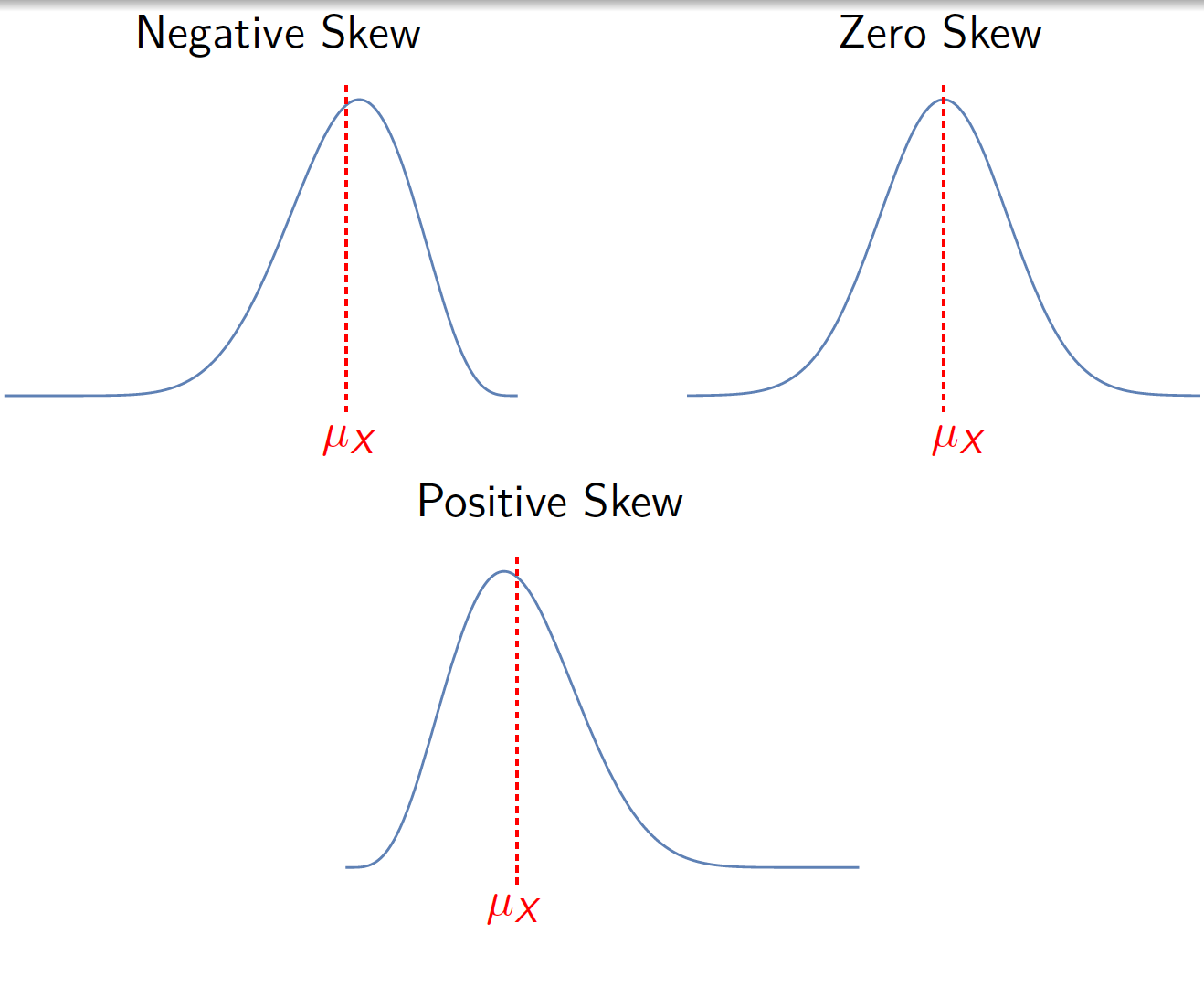
Skewness:
Beyond the location and dispersion it is desirable to know the distribution behaviour about the mean. One parameter of interest is the coefficient of asymmetry also known as skewness. This parameter is a measure of asymmetry of a probability function/density about the mean of the random variable. It is given by \[\gamma _{1}=\frac{E\left[ (X-\mu _{X})^{3}\right] }{Var\left( X\right) ^{3/2}% }=\frac{\mu _{3}}{\sigma _{X}^{3}}\]
Remarks:
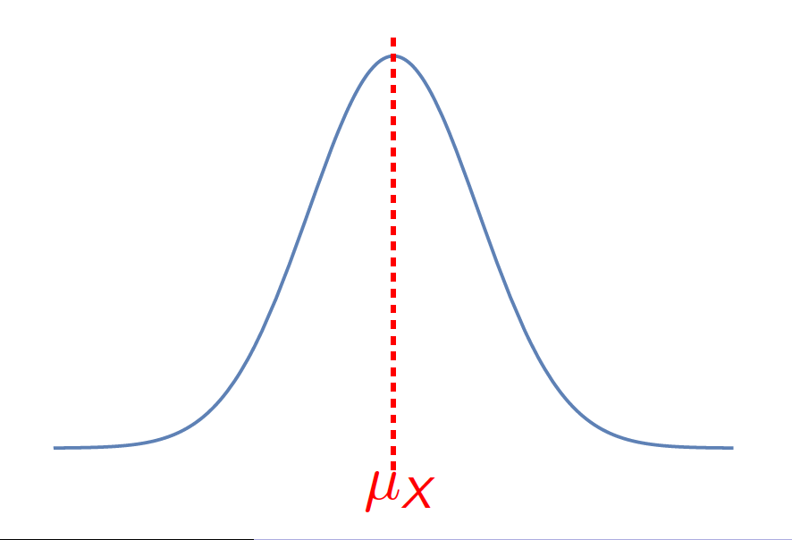
For discrete random variables a probability function is symmetric if \(% f_{X}\left( \mu _{x}-\delta \right) =f_{X}\left( \mu _{x}+\delta \right)\) for all \(\delta \in \mathbb{R}.\)
For continuous random variables the probability density function is symmetric if \(f_{X}\left( \mu _{x}-\delta \right) =f_{X}\left( \mu _{x}+\delta \right)\) for all \(\delta \in \mathbb{R}\)
Example 5.6 Let \(X\) be a discrete random variable with probability function given by \[f_{X}\left( x\right) =\left \{ \begin{array}{cc} 0.25 & ,\text{ for }x=-1 \\ 0.5 & ,\text{ for }x=0 \\ 0.25 & ,\text{for }x=1% \end{array}% \right. .\]
Note that \[\mu _{X}=E(X)=\left( -1\right) \times 0.25+\left( 0\right) \times 0.5+1\times 0.25=0\] and \[E(X^{3})=\left( -1\right) ^{3}\times 0.25+\left( 0\right) ^{3}\times 0.5+1^{3}\times 0.25.=0.\] Therefore, \(f_{X}\left( x\right)\) is symmetric about \(\mu _{X}=0\) and \(\gamma _{1}=0.\)
Remark: Note however that we can have \(\gamma _{1}=0,\) and the probability function/density is not symmetric about the mean, that is \(\gamma _{1}=0\) does not imply symmetry.
Example 5.7 Let \(X\) be a discrete random variable with probability function given by \[f_{X}\left( x\right) =\left \{ \begin{array}{cc} 0.1 & ,\text{ for }x=-3 \\ 0.5 & ,\text{ for }x=-1 \\ 0.4 & ,\text{for }x=2% \end{array}% \right. .\]
Note that \[\mu _{X}=E(X)=\left( -3\right) \times 0.1+\left( -1\right) \times 0.5+2\times 0.4=0.\] Since \(f_{X}\left( -1\right) \neq f_{X}\left( 1\right) ,\) this function is not symmetric around \(\mu _{X}=0\). However \[% E(X^{3})=\left( -3\right) ^{3}\times 0.1+\left( -1\right) ^{3}\times 0.5+2^{3}\times 0.4.=0,\] and consequently \(\gamma _{1}=0.\)
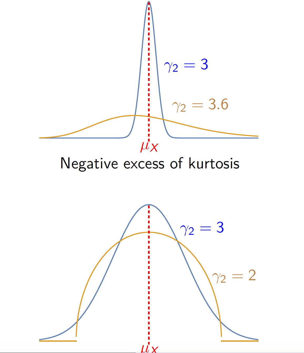
Kurtosis:
The kurtosis measures the “thickness” of the "tails" of the probability function/density or, equivalently, the “flattening” of the probability function/density in the central zone of the distribution.
\[\gamma _{2}=\frac{E\left[ (X-\mu _{X})^{4}\right] }{Var\left( X\right) ^{2}}=% \frac{\mu _{4}}{\sigma _{X}^{4}}.\]
The kurtosis of the normal distribution is \(3\). We use this distribution as reference, therefore we can define the excess of kurtosis as \[\gamma_2'=\frac{\mu _{4}}{\sigma _{X}^{4}}-3\]
6 Quantiles and Mode of A Distribution
Quantiles: Other parameters of interest are the quantiles of a (cumulative) distribution or quantiles of a random variable. Quantiles have the advantage that they exist even for random variables that do not have moments.
Definition: Let be \(X\) be random variable and \(\alpha \in \left( 0,1\right)\). The quantile of order \(\alpha\), \(q_{\alpha }\) is the smallest value among all points \(x\) in \(\mathbb{R}\) that satisfy the condition \[F_{X}\left( x\right) \geq \alpha .\]
Remarks:
If \(X\) is a discrete random variable \(q_{\alpha }\in D_{X}.\)
The quantile \(0.5\) is called the median of a (cumulative) the distribution function. It can also be interpreted as a centre of the distribution and therefore it is also considered a measure of location.
When the probability function/ density is symmetric the \(median=mean\).
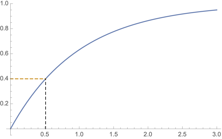
Example: Let \(X\) be a random variable such that \[F_{X}(x)=\begin{cases} 0,&x<0\\ 1-e^{-x},&xx\geq 0 \end{cases}\] What is the quantile of order \(0.4\)?
Solution:We can start by solving \[F_X(x)=0.4\Leftrightarrow x=-ln(0.6)\approx 0.5108\]
Let \(X\) be a discrete random variable such that \[X=\begin{cases} 1, & \text{if there is a success}\\ 0, &\text{otherwise} \end{cases}\text{ and } P(X=x)=\begin{cases} p,& \text{if }x=1\\ 1-p,& \text{if }x=0 \end{cases}.\] It follows that \[F_{X}\left( x\right) =\left \{ \begin{array}{cc} 0 & ,\text{ for }x<0 \\ 1-p & \text{for }0\leq x<1 \\ 1 & ,\text{ for }x\geq 1% \end{array}% \right.\]
Compute the quantile of order 0.5 when \(p=0.2\).
Compute the quantile of order 0.5 when \(p=0.6\).
Fix \(p=0.2\):
\(q_{0.5}\) which is the smallest value among all points \(x\) in \(\mathbb{R}\) that satisfy the condition \[F_{X}\left( x\right) \geq 0.5.\]
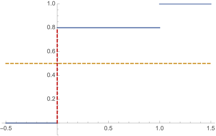
Therefore, \(q_{0.5}=0\).
Fix \(p=0.6\):
\(q_{0.5}\) which is the smallest value among all points \(x\) in \(\mathbb{R}\) that satisfy the condition \[F_{X}\left( x\right) \geq 0.5.\]
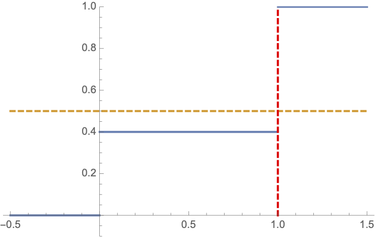
Therefore, \(q_{0.5}=1\).
Remarks:
The \(q_{\alpha }\) are called quartiles if \(\alpha =0.25\), \(0.5\), \(% 0.75.\) Therefore the first quartile is \(q_{0.25},\) the second quartile is \(% q_{0.5}\) and the third quartile is \(q_{0.75}\)
The \(q_{\alpha }\) are called deciles if \(\alpha =0.1\), \(0.2\),...,\(0.9\) . Therefore the first decile is \(q_{0.1},\) the second decile is \(q_{0.2}\), etc..
The \(q_{\alpha }\) are called percentiles if \(\alpha =\) \(0.01\), \(0.02\) ,…,\(0.99\). Therefore the first percentile is \(q_{0.01},\) the second percentile is \(q_{0.02}\), etc.
The interquartile range \(IQR=q_{0.75}-q_{0.25}\) is considered a measure of dispersion.
The mode: The mode of a random variable \(X\) or distribution is the value \(mo(X)\) that satisfies the condition \(f_{X}\left( mo(X)\right) \geq f_{X}\left( x\right) ,\) for all \(x\in \mathbb{R}\), where \(f_{X}\left( x\right)\) is the probability function in the case of discrete random variables and it is the probability density function in the case of continuous random variables.
Remarks:
The mode can also be interpreted as a centre of the distribution and therefore it is also considered a measure of location.
In the case of discrete random variable the mode is the most frequent value.
The mode does not have to be unique.
If the variable probability distribution/density is symmetric and has only one mode, then the mode equals the median and the mean.
Example 6.1 Let \(X\) be a discrete random variable such that \[X=\begin{cases} 1, & \text{if there is a success}\\ 0, &\text{otherwise} \end{cases}\text{ and } P(X=x)=\begin{cases} p,& \text{if }x=1\\ 1-p,& \text{if }x=0 \end{cases}.\]
Fix \(p=0.2\):
It follows that \(mo(X)=\arg\max_{x\in \mathbb{R}}P(X=x)=0.\)
Fix \(p=0.6\):
It follows that \(mo(X)=\arg\max_{x\in \mathbb{R}}P(X=x)=1.\)
Fix \(p=0.5\):
It follows that \(mo(X)=\arg\max_{x\in \mathbb{R}}P(X=x)=0\text{ and } 1.\)
In this case, there are two modes \(mo(X)=0\) and \(% mo(x)=1.\)
Example 6.2 Let \(X\) be a continuous random variable with density function \[f_{X}\left( x\right) =\left \{ \begin{array}{cc} x & 0<x\leq 1\\ 2-x & 1<x< 2 \end{array}% \right.\] Compute the mode.
Solution: Since \(f_{X}\left( x\right) <1\) for \(x\in(0,2)\setminus\{1\}\) and \(f_X(1)=1\) the the mode is given by \(mo(X)=1\) because \(x=1\) maximizes the function \(f\).
Example 6.3 Let \(X\) be a continuous random variable with density function \[f_{X}\left( x\right) =\left \{ \begin{array}{cc} 2x, & 0<x<1\\ 0,&\text{otherwise} \end{array}% \right.\] There is no mode because the density function does not have a maximum.
7 Moment Generating Functions
The moment generating function: The moment generating function is an important function in probability because it defines uniquely the distribution function (when the moment generating function is properly defined).
Definition: The moment generating function of a discrete random variable is given by \[M_{X}\left( t\right) =E\left( e^{tX}\right) =\sum_{x\in D_{X}}e^{tx}\times f_{X}\left( x\right) =\sum \limits_{i=1}^{\infty }e^{tx_{i}}\times f_{X}\left( x_{i}\right) ,\text{ }\] provided that it is finite.
Definition: The moment generating function of a continuous random variable is given by \[M_{X}\left( t\right) =E\left( e^{tX}\right) =\int_{-\infty }^{+\infty }e^{tx}f_{X}(x)dx..\] provided that it is finite.
Remarks on the moment generating function (m.g.f.):
The m.g.f. may not exist.
If \(X\) is a discrete random variables and \(D_{X}\) is finite, then there is always a m.g.f.;
The moment generating function is a function of \(t\) not \(X\);
If there is a m.g.f., then there are moments of every order. The reverse is not true.
A distribution which has no moments – or has only the first \(k\) moments – does not have a m.g.f..
The moment generating function is used to calculate the moments.
The m.g.f. uniquely determines the distribution function. That is, if two random variables have the same m.g.f., then the cumulative distribution functions of the random variables coincide, except perhaps at a finite number of points.
Theorem: Let \(X\) be a random variable with moment generating function \(M_X\) defined. Then, \[\left. \frac{d^{r}M_{X}\left( t\right) }{dt^{r}}\right \vert _{t=0}=\mu _{r}^{\prime }=E\left[ X^{r}\right] ,\text{ }r=1,2,3,...\]
Remark: This result allows us to compute the raw moment of \(X\) of order \(k\) by computing the \(k^{\text{th}}\) derivative and evaluate it at the point \(0\).
Example: Let \(X\) be a random variable such that \[f_X(x)=\begin{cases} 0.2,&x=0,3\\ 0.5,&x=1\\ 0.1,&x=2\\ 0,&\text{otherwise} \end{cases}\] By definition, \[E(X)=\sum_{x=0}^3xf_X(x)=0\times 0.2+1\times 0.5+2\times 0.1+3\times 0.2=1.3.\]
By using the moment generating function, we have \[M_X(t)=\sum_{x=0}^3e^{tx}f_X(x)=0.2(1+e^{3t})+0.5e^{t}+0.1e^{2t}.\] Therefore, \[M_X'(t)=0.6e^{3t}+0.5e^{t}+0.2e^{2t},\] and, consequently, \[E(X)=M_X'(0)=1.3.\]
Example 7.1 Let \(X\) be a discrete random variable such that \[X=\begin{cases} 1, & \text{if there is a success}\\ 0, &\text{otherwise} \end{cases}\text{ and } P(X=x)=\begin{cases} p,& \text{if }x=1\\ 1-p,& \text{if }x=0 \end{cases}.\] The moment generating function \(M_X(t)\) is given by \[M_X(t)=E(e^{tX})=(1-p)e^{0\times t}+p e^{t\times 1}=(1-p)+p e^{t}.\] The derivative of \(M_X(t)\) in \(t\) is given by \[\frac{\partial}{\partial t}M_X(t)=p e^{t}.\] Therefore, \[E(X)=\frac{\partial}{\partial t}M_X(t)\Big\vert_{t=0}=p\]
Example: Let \(X\) be a continuous random variable with density function \[f_{X}\left( x\right) =\left \{ \begin{array}{cc} 0 & ,\text{ for }x<0 \\ \lambda e^{-\lambda x} & \text{for }x\geq 0% \end{array}% \right.\]
\[\begin{aligned} M_{X}\left( t\right) &=&E\left( e^{tX}\right) =\int_{0}^{+\infty }\lambda e^{(t-\lambda)x}dx \\ &=&\lambda\lim_{z\rightarrow \infty }\int_{0}^{z}e^{(t-\lambda)x}dx=\lambda\lim_{z\rightarrow \infty }\left[ \frac{e^{(t-\lambda)x}}{t-\lambda}\right] _{x=0}^{x=z} \\ &=&-\frac{\lambda}{t-\lambda}, \end{aligned}\]
provided that \(t<\lambda.\) Now \[\frac{dM_{X}\left( t\right) }{dt}=\frac{d\left( -\frac{\lambda}{t-\lambda}\right) }{dt}=% \frac{\lambda}{\left( t-\lambda\right) ^{2}}\] and, consequently, \[E(X)=\left. \frac{dM_{X}\left( t\right) }{dt}\right \vert _{t=0}=\frac{1}{\lambda}.\]
Proposition: Let \(X\) be a random variable such that \(M_X\) is its moment generating function. For \(a,b\in\mathbb{R}\), \[M_{bX+a}\left( t\right) =E\left[ e^{\left( bX+a\right) t}\right] =e^{at}M_{X}\left( bt\right).\]
Proposition: Let \(X_i\), with \(i=1,\cdot,n\) be independent random variables such that its moment generating function is given by \(M_{X_i}\). The moment generating function of a sum of independent random variables \(S_{n}=\sum_{i=1}^{n}X_{i}\) equals the product of their m.g.f.(s). \[M_{S_{n}}\left( t\right) =M_{X_{1}}\left( t\right) \times M_{X_{2}}\left( t\right) \times ...\times M_{X_{n}}\left( t\right)\].