2. Random Variables
1 Random Variables
Random variable, informally, is a variable that takes on numerical values and has an outcome that is determined by an experiment.
Random Variable: Let \(S\) be a sample space with a probability measure. A random variable (or stochastic variable) \(X\) is a real-valued function defined over the elements of S. \[\begin{aligned} X:& S\to\mathbb{R}\\ &s\to X(s)\end{aligned}\]
Important convention: Random variables are always expressed in capital letters. On the other hand, particular values assumed by the random variables are always expressed by lowercase letters.
Remark: Although a random variable is a function of \(s\); usually we drop the argument, that is we write \(X\); rather than \(X(s)\).
Remark:
Once the random variable is defined, R is the space in which we work with;
The fact that the definition of a random variable is limited to real-valued functions does not impose any restrictions;
If the outcomes of an experiment are of the categorical type, we can arbitrarily make the descriptions real-valued by coding the categories, perhaps by representing them with the numbers.
Example 1.1 One flips a coin and observes if a head or tail is obtained. $$$$
Sample Space: \[S=\{H,T\}\]
Random Variable: \[X:S\to\{0,1\} \text{ with } X(H)=0\text{ and } X(T)=1.\]
The definition of random variable does not rely explicitly on the concept of probability, it is introduced to make easier the computation of probabilities. Indeed, if \(B\subset \mathbb{R}\), then \[\begin{aligned} P(X\in B)=P(A),\quad\text{where}\quad A=\{s\in S: X(s)\in B\}\end{aligned}\]
Is now clear that: \[\begin{aligned} P(X\in B)=1-P(X\notin B).\end{aligned}\] In particular, \[\begin{aligned} P(X\leq x)=1-P(X>x);\\ P(X< x)=1-P(X\geq x)\end{aligned}\]
2 Cumulative Distribution Function
2.1 Cumulative distribution function
Let \(X\) be a random variable. The cumulative distribution function \(F_X\) is a real function of real variable given by: \[F_X(x)=P(X\leq x)=P(X\in(-\infty,x])\]
Properties of CDFs:
\(0\leq F_{X}\left( x\right) \leq 1;\)
\(F_{X}\left( x\right)\) is non-decreasing: \(\forall \Delta _{x}>0:\) \(% F_{X}\left( x\right) \leq F_{X}\left( x+\Delta _{x}\right) .\)
\(\lim\limits_{x\rightarrow -\infty }F_{X}\left( x\right) =0\) and \(% \lim\limits_{x\rightarrow +\infty }F_{X}\left( x\right) =1.\)
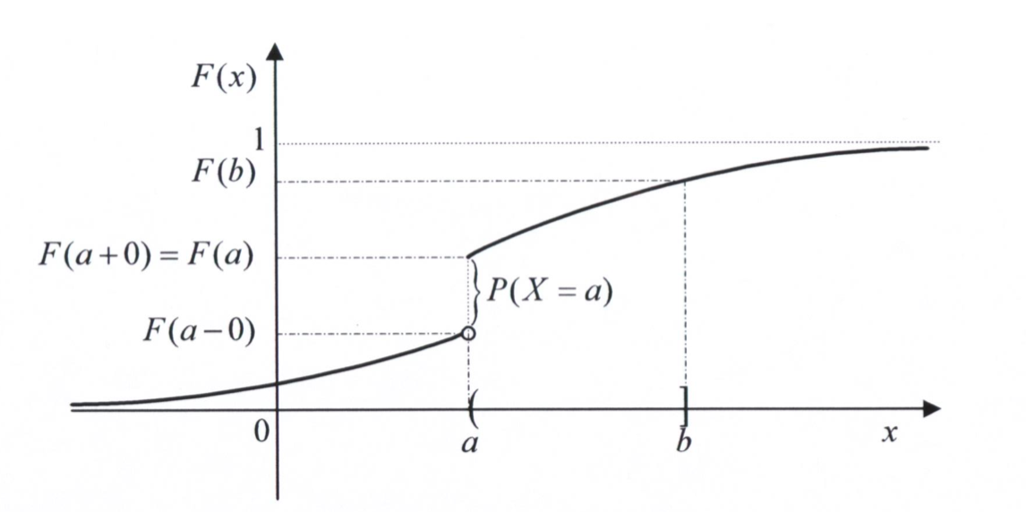
\(P\left( a<X\leq b\right) =F_{X}\left( b\right) -F_{X}\left( a\right) ,\) for \(b>a\)
\(\lim\limits_{x\rightarrow a^{+}}F_{X}\left( x\right) =F_{X}(a);\) therefore \(% X\) is right continuous
\(P(X=a)=F_{X}\left( a\right) -\lim\limits_{x\rightarrow a^{-}}F_{X}\left( x\right)\) for any real finite number.
Example 2.1 One flips a coin and observes if a head or tail is obtained.
Sample Space: \(S=\{H,T\}\)
Random Variable: \(X:S\to\{0,1\} \text{ with } X(H)=0\text{ and } X(T)=1.\)
\(X\) counts the number of tails obtained.
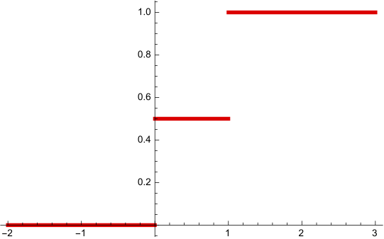
It is easy to see that: \(P(X=0)=1/2\), \(P(X=1)=1/2\). Since we have \(F_X(x)=P(X\leq x)\), then
\[ \begin{aligned} F_X(x)=&P(X\leq x)\\ =&\begin{cases} 0,& x<0\\ \frac{1}{2}, & 0\leq x< 1\\ 1,& x\geq 1 \end{cases} \end{aligned} \]
Example 2.2 One flips a coin twice and counts the number of tails obtained.
Sample Space: \(S=\{(H,T), (H,H), (T,H), (T,T)\}\)
Random Variable:
\(X:S\to\{0,1,2\}\) \(X((H,T))=1, \, X((H,H))=0\), \(X((T,H))=1, X((T,T))=2.\)
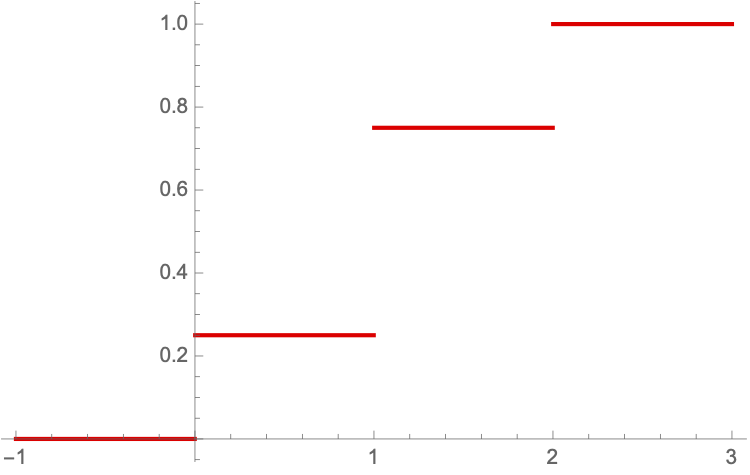
It is easy to see that: \(P(X=s)=1/4\), for \(s=0,2\) and \(P(X=1)=1/2\). Since we have \(F_X(x)=P(X\leq x)\), then
\[F_X(x)=\begin{cases} 0,& x<0\\ \frac{1}{4}, & 0\leq x< 1\\ 3/4,& 1\leq x <2\\ 1, & x\geq 2 \end{cases}\]
Further properties:
\(P(X<b)=F_{X}\left(b\right)-P(X=b)\)
\(P(X>a)=1-F_{X}(a)\)
\(P(X\geq a)=1-F_{X}\left( a\right)+P(X=a)\)
\(P\left( a<X<b\right) =F_{X}\left( b\right) -F_{X}\left( a\right)-P(X=b)\)
\(P\left( a\leq X<b\right) =F_{X}\left( b\right) -F_{X}\left( a\right)-P(X=b) +P(X=a)\)
\(P\left( a\leq X\leq b\right) =F_{X}\left( b\right)-F_{X}\left( a\right)+P(X=a)\)
Prove the previous properties!
Proof: To prove that \(P(X\geq a)=1-F_{X}\left( a\right)+P(X=a)\), one notes that: \[\begin{aligned} P(X\geq a)&=1-P(X<a)=1-P(X\leq a)+P(X=a)\\ &=1-F_X(a)+P(X=a)\end{aligned}\]
The set of discontinuities of the cumulative distribution function \(D_{X}\) is given by \(D_{X}=\left \{ x\in \mathbb{R}: P(X=x)>0\right \} .\) Note that by property 6 this the same as
\[ D_{X}=\left \{ a\in \mathbb{R}:F_{X}\left( a\right) -\lim_{x\rightarrow a^{-}}F_{X}\left( x\right) >0\right \} . \]
2.2 Types of random variables
Discrete Random Variable: \(X\) is a discrete random variable if \[\begin{aligned} D_X\neq \emptyset\quad\text{and}\quad\sum_{x\in D_x}P(X=x)=1.\end{aligned}\]
Continuous Random Variable: \(X\) is a continuous random variable if \(D_X= \emptyset\) and there is a non-negative function \(f\) such that \[\begin{aligned} F_X(x)=\int_0^xf(s)ds.\end{aligned}\]
Mixed Random Variable: \(X\) is a mixed random variable if
\[ \begin{aligned} &D_X\neq \emptyset,\quad\sum_{x\in D_x}P(X=x)<1\quad\text{and}\\ &\exists \lambda\in(0,1)\text{ such that }F_X(x)=\lambda F_{X_1}(x)+(1-\lambda)F_{X_2}(x) \end{aligned} \]
where \(X_1\) is a discrete random variable and \(X_2\) is a continuous random variable.
3 Discrete Random Variables
\(X\) is a discrete random variable if
\[\begin{aligned} D_X\neq \emptyset\quad\text{and}\quad\sum_{x\in D_x}P(X=x)=1. \end{aligned}\] Additionally, the function \(f_X:\mathbb{R}\to[0,1]\) defined by
\[f_X(x)=\begin{cases} P(X=x),&x\in D_X\\ 0,&x\in D_X \end{cases}. \] is called the probability mass function (pmf).
Theorem: A function can serve as the probability function of a discrete random variable \(X\) if and only if its values, \(f_{X}(x)\), satisfy the conditions
\(0\leq f_{X}(x_{j})\leq 1,\) \(j=1,2,3,...\)
\(\sum \nolimits_{j=1}^{\infty }f_{X}(x_{j})=1.\)
For discrete random variables, the cumulative distribution function (cdf) is given by :
\[ F_{X}\left( x\right) =P\left( X\leq x\right) =\sum_{x_{j}\leq x}f_{X}(x_{j}). \]
Generally,
\[ P(X\in B)=\sum_{x_{j}\in B\cap D_X}f_{X}(x_{j}). \]
Theorem: If the range of a random variable X consists of the values \(x_1 <x_2 <\cdots<x_n\), then \[\begin{aligned} f_X(x_1)=F_X(x_1),\quad\text{and}\quad f_X(x_i)=F_X(x_i)-F_{X}(x_{i-1}), \end{aligned}\] \(i=2,3,\cdots n.\)
Example 3.1 Check whether the function given by \(f(x)=\frac{x+2}{25}\), for \(x=1,2,3,4,5\) can serve as the probability function of a discrete random variable \(X\). Compute the cumulative distribution function of \(X\).
4 Continuous Random Variables
4.1 Continuous Random Variables
\(X\) is a continuous random variable if \(D_X= \emptyset\) and there is a function \(f_X:\mathbb{R}\to\mathbb{R}_0^+\) such that
\[ \begin{aligned} F_X(x)=\int_{-\infty}^xf_X(s)ds. \end{aligned} \]
Additionally, \(f_X\) is called the probability density function.
Remark:
Continuity of \(F_X\) is necessary, but not sufficient to guarantee that \(X\) is a continuous random variable;
Note that \(P(X\in D_{X})=P(X\in\emptyset)=0\);
The function \(f_{X}\) provides information on how likely the outcomes of the random variable are.
4.2 Probability Density Function
Theorem. A function can serve as a probability density function of a continuous random variable \(X\) if its values, \(f_{X}(x)\), satisfy the conditions:
\(f_{X}(x)\geq 0\) for \(-\infty <x<+\infty\);
\(\int_{-\infty }^{+\infty }f_{X}(x)dx=1\).
Example 4.1 Let \(X\) be a continuous random variable with a probability density function \(f_X\) given by
\[ f_X(x)=\begin{cases} 1/5, &x\in[3,a]\\ 0, &x\in\mathbb{R}\setminus[3,a] \end{cases} \]
Find the value of the parameter \(a\).
According to the previous theorem, we know that \[ \begin{aligned} &f_X(x)\geq 0, \text{ for } -\infty <x<+\infty\\ &\int_{-\infty }^{+\infty }f_{X}(x)dx=1 \end{aligned} \]
From the second condition, we get that
\(\frac{a}{5}-\frac{3}{5}=1\Leftrightarrow a=8\).
Theorem. If \(f_{X}(x)\) and \(F_{X}(x)\) are the values of the probability density and the distribution function of \(X\) at \(x\), then \[ \begin{aligned} P(a &\leq X\leq b)=F_{X}(b)-F_{X}(a) =\int \nolimits_{a}^{b}f_{X}(t)dt \end{aligned} \]
for any real constants \(a\) and with \(a\leq b\), and
\[ f_{X}(x)=\frac{dF_{X}(x)}{dx},\quad\text{almost everywhere.} \]
Remarks:
At the points \(x\) where there is no derivative of the CDF, \(F_X\), it is agreed that \(f_{X}(x)=0\). In fact, it does not matter the value that we give to \(f_{X}(x)\) as it does not affect the computation of \(F_{X}\).
The probability density function is not a probability and therefore it can assume values bigger than one.
If \(X\) is a continuous random variable \[ P(X=a)=\int \nolimits_{a}^{a}f_{X}(t)dt=0. \]
Example 4.2 Consider the continuous random variable \(X\) with a probability density function \(f_X\) and cumulative distribution function given by \[ f_X(x)=\begin{cases} 0,&x<0\\ 4x, &0\leq x\leq \frac{1}{2}\\ 4-4x, &\frac{1}{2}\leq x\leq 1\\ 0,&x>1 \end{cases} \]
Cumulative density function:
\[ F_X(x)=\begin{cases} 0,& x<0\\ 2x^2,&0\leq x< \frac{1}{2}\\ -1 + 4 x -2x^2,&\frac{1}{2}\leq x< 1\\ 1,& x\geq 1 \end{cases} \]
Is this function \(F_X\) differentiable?
Theorem: If \(X\) is a continuous random variable and \(a\) and \(b\) are real constants with \(a\leq b\), then \[ \begin{aligned} P(a &\leq &X\leq b)=P(a\leq X<b) \\ &=&P(a<X\leq b) \\ &=&P(a<X<b) \end{aligned} \]
Proof: To prove the previous theorem one needs notice that: \[ \begin{aligned} P(a \leq X\leq b)=&P(a< X<b)+P(X=a)+P(X=b) \\ =&P(a<X\leq b)+P(X=a) \\ =&P(a\leq X<b)+P(X=b) \end{aligned} \]
Additionally, for \(c=a\) or \(c=b\) we have
\[ \begin{aligned} P(X=c)=P(c& \leq X\leq c)=\int \nolimits_{c}^{c}f_{X}(t)dt=0 \end{aligned} \]
Remark: The previous inequalities are not necessarily true for discrete random variables.
5 Mixed random variables
Mixed Random Variable: \(X\) is a mixed random variable if
\[ \begin{aligned} &D_X\neq \emptyset,\quad\sum_{x\in D_x}P(X=x)<1\quad\text{and}\\ &\exists \lambda\in(0,1)\text{ tal que }F_X(x)=\lambda F_{X_1}(x)+(1-\lambda)F_{X_2}(x) \end{aligned} \]
where \(X_1\) is a discrete r.v. and \(X_2\) is a continuous r.v..
Example 5.1 A company has received 1 million € to invest in a new business. With probability \(\frac 1 2\), the firm does nothing but with probability \(\frac 1 2\) the money is invested. If it does not invest the money, \(1\) million € is kept. Otherwise, the firm gets back a random amount uniformly distributed between \(0\) and \(3\) million €.
Let \(X\) be the following random variable: \[ X=``\text{Amount received by the company in millions}" \] What type of random variable is \(X\)?
\[ S=[0,3]\quad\text{and}\quad X= \begin{cases} 1,& \text{with probability } \frac 1 2 \text{ (Scenario 1)}\\ [0,3],& \text{with probability } \frac 1 2 \text{ (Scenario 2)} \end{cases} \]
\(X\) is not a discrete r.v. because it takes values in a continuous set;
\(X\) is not a continuous random variable because \(P(X=1)=1/2\) (For continuous random variables the probability to take one single point is equal to \(0\)).
\(X\) is a mixed random variable?
We can define two random variables:
\[ \begin{aligned} X_1=&``\text{Amount received by the}\\ &\text{company in millions in S1}" \end{aligned} \]
\[ \begin{aligned} \hspace{-0.5cm} X_2=``\text{Amount received by the}\\ \text{company in millions in S2}" \end{aligned} \]
Since \(P(X_1=1)=1\), then \[ F_{X_1}(x)=\begin{cases} 0,&x<1 \\ 1,&x\geq 1 \end{cases} \]
On the other hand, in scenario 2, the firm gets back a random amount uniformly distributed between \(0\) and \(3\) million €. Therefore,
\[ f_{X_2}(x)=\begin{cases} \frac{1}{3},&x\in[0,3]\\ 0,& \text{otherwise} \end{cases},\quad\text{and}\quad F_{X_2}(x)=\begin{cases} 0,&x<0\\ \frac{x}{3},&0\leq x<3\\ 1,& x\geq 3, \end{cases} \]
Since S1 holds with probability \(\frac{1}{2}\) and S2 holds with probability \(\frac{1}{2}\), we have that
\[ \begin{aligned} F_X(x)&=\frac{1}{2}F_{X_1}(x)+\frac{1}{2}F_{X_2}(x)=\begin{cases} 0,&x<0\\ \frac{x}{6},&0\leq x<1\\ \frac{1}{2}+\frac{x}{6},&1\leq x<3\\ 1,& x\geq 3, \end{cases} \end{aligned} \]
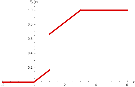
\(D_X=\{1\}\), because
\[ \begin{aligned} \hspace{-1cm} &F_X(1)-F_X(1^-)=\frac{2}{3}-\frac{1}{2}\\ &=\frac{1}{2}=P(X=1)<1 \end{aligned} \]
Exercise: Let
\[ F_{X} \left( x \right) = \left\{ \begin{array}{cc} 0 & x<0 \\ \frac{1}{12}+\frac{3}{4}\left( 1-e^{-x}\right) & 0\leq x<1 \\ \frac{1}{4}+\frac{3}{4}\left( 1-e^{-x}\right) & x\geq 1 \end{array} \right. , \]
Compute \(P(X=0),\) \(P(X=1),\) \(P\left( 0.5<X<1\right)\) and \(P\left( 0.5<X<2\right)\).
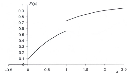
Answer: \[ \begin{aligned} &P(X=0)=\frac{1}{12},\quad P(X=1)=\frac{2}{12}\\ &P\left( 0.5<X<1\right)=F_{X}(1)-F_{X}(0.5)-P(X=1)=\frac{3}{4}\left(e^{-0.5}-e^{-1}\right)\\ &P\left(0.5<X<2\right) = F_{X}(2)-F_{X}(0.5)=\frac{2}{12}+\frac{3}{4}\left(e^{-0.5}-e^{-2}\right) \end{aligned} \]
6 The Distribution of Functions of Random Variables
Motivation: Assume that the random variable \(D\) represents the demand of a given product in a store. The profit of this store is represented by the random variable \(L=4D-5\). If the probability function of \(D\) is given by
\[ P(D=d)=\begin{cases} 0.3,&d=0\\ 0.2,&d=1\\ 0.3,&d=2\\ 0.2,&d=3 \end{cases}, \] what is the probability of having \(L>2\)?
\[ P(L>2)=P\left(D>\frac{7}{4}\right)=P(D=2)+P(D=3)=0.5 \] Since \(L\) is a random variable, it should be possible to find its distribution. How to do it?
Let \(X\) be a known random variable with known cumulative distribution function \(% F_{X}(x)\).
Consider a new random variable \(Y=g(X)\), where \(g:\mathbb{R}\rightarrow \mathbb{R}\) is a known function. Let \(% F_{Y}(y)\) be the cumulative distribution function of \(Y.\) How can we derive \(F_{Y}(y)\) from \(F_{X}(x)?\).
The derivation of \(F_{Y}(y)\) is based on the equality
\[ \begin{aligned} F_{Y}(y)=P(Y\leq y)=P(g(X)\leq y)=P(X\in A_{y}^{\ast }) \end{aligned} \] where \(A_{y}^{\ast }=\left \{ x:g(x)\leq y\right \}\)
Example 6.1 Derive the cumulative distribution functions of \(Y=aX+b,\) where \(a>0\) and \(Z=X^{2}\).
- \(Y=aX+b\)
\[ \begin{aligned} F_Y(y)&=P(Y\leq y)=P(aX+b\leq y)\\ &=P\left(X\leq\frac{y-b}{a}\right)=F_X\left(\frac{y-b}{a}\right) \end{aligned} \]
- \(Z=X^2\)
For \(z\geq 0\),
\[ \begin{aligned} F_Z(z)&=P(Z\leq z)=P(X^2\leq z)\\ &=P\left(-\sqrt{z}\leq X\leq \sqrt{z}\right)\\ &=F_X\left(\sqrt{z}\right)-F_X\left(-\sqrt{z}\right)+P(X=-\sqrt{z}) \end{aligned} \]
6.1 Functions of Continuous Random Variables
Assume that in the previous example \(X\) is a continuous random variable such that
\[ F_X(x)= \begin{cases} 0,&x<0\\ x,&0\leq x<1\\ 1,&x\geq 1 \end{cases}, \]
then the following holds:
- \(Y=aX+b\)
\[ \begin{aligned} F_Y(y)=&F_X\left(\frac{y-b}{a}\right)=\begin{cases} 0,&\frac{y-b}{a}<0\\ \frac{y-b}{a},&0\leq \frac{y-b}{a}<1\\ 1,&\frac{y-b}{a}\geq 1 \end{cases}\\ =&\begin{cases} 0,&{y<b}\\ \frac{y-b}{a},&b\leq y<a+b\\ 1,&y\geq a+b \end{cases} \end{aligned} \]
Example 6.2 Assume that in the previous example \(X\) is a continuous random variable such that
\[ F_X(x)=\begin{cases} 0,&x<0\\ x,&0\leq x<1\\ 1,&x\geq 1 \end{cases}, \] then the following holds:
\(Z=X^2\)
If \(z<0\) then \(F_Z(z)=P(Z\leq z)=0\). When \(z\geq 0\)
\[ \begin{aligned} F_Z(z)&=F_X\left(\sqrt{z}\right)-F_X\left(-\sqrt{z}\right)+\underbrace{P(X=-\sqrt{z})}_{=0, \text{ because } X \text{ is continuous}}\\ &=F_X\left(\sqrt{z}\right)-\underbrace{F_X\left(-\sqrt{z}\right)}_{=0 \text{ because }-\sqrt{z}\text{ is negative}}\\ &=\begin{cases} 0,&z<0\\ \sqrt{z},&0\leq z<1\\ 1,&z\geq 1 \end{cases} \end{aligned} \]
6.2 Functions of Discrete Random Variables
When \(X\) is a discrete random variable, it is easier to find the distribution of \(Y=g(X)\). In this case, we will derive the probability function.
Let \(D_{X}=\left \{ x_{1},x_{2},x_{3}...\right \}\) be the set of discontinuities of \(F_{X}(x),\) then \(D_{Y}=\left \{ g(x_{1}),g(x_{2}),g(x_{3})...\right \}\) is the set of discontinuities of \(F_{Y}(y).\)
The probability function of \(Y\) is given by
\[ \begin{aligned} f_{Y}(y)&=P(Y=y)=P(g(X)=y)\\ &=P(X\in \{x\in D_X:g(x)=y\})\\ &=\sum_{x_{i}\in \{x\in D_X:g(x)=y\}}f(x_{i}) \end{aligned} \]
Example 6.3 Consider the discrete random variable \(X\) with probability function
| x | -2 | -1 | 0 | 1 | 2 |
| \(\mathbf{f_X(x)}\) | 12/60 | 15/60 | 10/60 | 6/60 | 17/60 |
Let \(Y=X^{2},\) what is \(f_{Y}(y)?\)
Firstly: The set of discontinuities \(D_Y\) is \(D_{Y}=\left \{ 0,1,4\right \}\)
| x | -2 | -1 | 0 | 1 | 2 |
| \(\mathbf{y=x^2}\) | 4 | 1 | 0 | 1 | 4 |
Consequently
\(f_{Y}(0)=P(Y=0)=P(X^{2}=0)=P(X=0)=\frac{10}{60}\).
\(f_{Y}(1)=P(Y=1)=P(X^{2}=1)=P(X=1)+P(X=-1)=6/60+15/60=21/60.\)
\(f_{Y}(4)=P(Y=4)=P(X^{2}=4)=P(X=2)+P(X=-2)=17/60+12/60=29/60.\)